ꯌꯨꯗꯦꯃꯣꯅꯁꯤꯡ
ꯐꯤꯖꯤꯛꯁꯀꯤ ꯁꯤꯟꯃꯤꯁꯤꯡ, ꯀꯦꯁꯅꯥ ꯂꯩꯈꯤꯕ ꯀꯦꯁꯤꯅꯣꯒꯤ ꯆꯛꯔ ꯑꯃꯥ, ꯑꯃꯁꯨꯡ ꯇꯦꯕꯜꯗ ꯁꯥꯒꯠꯇꯨꯅ ꯆꯠꯄ ꯌꯥꯕ ꯃꯈꯥꯏꯅ ꯑꯄꯤꯀꯄ ꯀꯝꯞꯌꯨꯇꯔ ꯑꯃꯥ꯫

1976ꯗꯒꯤ 1981 ꯐꯥꯑꯣꯕ ꯁꯥꯟꯇꯥ ꯀ꯭ꯔꯨꯖꯇ ꯂꯩꯕ ꯐꯤꯖꯤꯛꯁꯀꯤ ꯁꯤꯟꯃꯤ ꯒ꯭ꯔꯨꯞ ꯑꯃꯅ ꯗꯤꯖꯤꯇꯦꯜ ꯀꯝꯞꯌꯨꯇꯔꯁꯤꯡ ꯁꯦꯃꯈꯤ; ꯃꯈꯣꯌꯅ ꯕꯣꯜ ꯑꯃꯁꯨꯡ ꯔꯣꯇꯔꯒꯤ ꯃꯇꯝ ꯂꯧꯈꯤ ꯑꯃꯁꯨꯡ ꯕꯦꯠ ꯍꯧꯖꯤꯛꯁꯨ ꯍꯥꯡꯗꯨꯅ ꯂꯩꯔꯤꯉꯩꯗ ꯆꯛꯔꯒꯤ ꯁꯦꯛꯇꯔ ꯑꯃꯥ ꯍꯥꯌꯈꯤ꯫ ꯃꯈꯣꯌꯒꯤ ꯇꯦꯁ꯭ꯇꯁꯤꯡꯅ 44%ꯒꯤ ꯑꯦꯗꯚꯥꯟꯇꯦꯖ ꯑꯃꯥ ꯋꯥꯁꯀꯈꯤ ꯑꯃꯁꯨꯡ ꯑꯍꯥꯅꯕ ꯁꯥꯡꯕ ꯁꯦꯁꯟ ꯑꯃꯅ 25% ꯃꯇꯧ ꯄꯤꯈꯤ꯫ ꯍꯥꯔꯗꯋꯦꯌꯔ ꯑꯗꯨ ꯂꯦꯞꯇꯅꯥ ꯐꯠꯇꯈꯤ, ꯈꯣꯡꯎꯞ ꯑꯃꯗ ꯁꯦꯃꯈꯤꯕ ꯚꯔꯁꯟ ꯑꯗꯨ 1981ꯗ ꯏꯂꯦꯛꯠꯔꯤꯛꯀꯤ ꯅꯣꯏꯖꯅ ꯃꯥꯏꯊꯤꯍꯅꯈꯤ, ꯑꯃꯁꯨꯡ ꯃꯈꯣꯌꯅ ꯗꯣꯂꯥꯔ ꯂꯤꯁꯤꯡ ꯈꯔꯈꯛ ꯃꯥꯏꯄꯥꯛꯈꯤ꯫
ꯂꯥꯁ ꯚꯦꯒꯥꯁꯀꯤ ꯕꯥꯔ ꯑꯃꯗ ꯊꯣꯔꯀꯈꯤꯕ ꯋꯥꯈꯜ, 1975
Doyne Farmer recalls forming Eudaemonic Enterprises with Norman Packard and friends while in graduate school. They hoped roulette winnings would fund a science commune. Their idea depended on measuring the physical game, rather than changing stakes after wins or losses.
ꯐꯤꯖꯤꯛꯁ ꯂꯦꯕꯇ ꯆꯛꯔ ꯑꯃꯥ
1976ꯒꯤ ꯂꯩꯃꯥꯏ ꯊꯥꯗ ꯐꯥꯔꯃꯔ ꯑꯃꯁꯨꯡ ꯗꯦꯟ ꯕ꯭ꯔꯥꯎꯅꯅ ꯔꯤꯅꯣꯗ ꯂꯩꯕ ꯋꯔꯀꯁꯣꯞ ꯑꯃꯗ ꯑꯃꯨꯛ ꯍꯟꯅꯥ ꯁꯦꯃꯗꯣꯀꯈꯤꯕ ꯀꯦꯁꯤꯅꯣꯒꯤ ꯆꯛꯔ ꯑꯃꯒꯤꯗꯃꯛ ꯀꯦꯁꯅꯥ $1,500 ꯄꯤꯈꯤ, ꯃꯁꯤ ꯐ꯭ꯔꯥꯇꯔꯅꯤꯇꯤ ꯄꯥꯔꯇꯤꯒꯤꯗꯃꯛꯅꯤ ꯍꯥꯌꯗꯨꯅ꯫ ꯊꯥ ꯀꯌꯥꯒꯤ ꯃꯅꯨꯡꯗ ꯃꯈꯣꯌꯅ ꯃꯁꯤ ꯅꯨꯃꯤꯗꯥꯡ ꯌꯨꯅꯤꯚꯔꯁꯤꯇꯤꯒꯤ ꯇꯝꯕꯒꯤ ꯂꯦꯕꯇ ꯄꯨꯈꯤ ꯑꯃꯁꯨꯡ ꯏꯅꯐ꯭ꯔꯥꯔꯦꯗ ꯁꯦꯟꯁꯔꯁꯤꯡ, ꯌꯨꯃꯗ ꯁꯦꯝꯕ ꯏꯂꯦꯛꯠꯔꯣꯅꯤꯛ ꯘꯔꯤ ꯑꯃꯥ ꯑꯃꯁꯨꯡ ꯕꯣꯜꯅ ꯃꯦꯇꯦꯜ ꯁꯣꯛꯄꯒꯤ ꯈꯣꯟꯖꯦꯂꯅ ꯆꯂꯥꯏꯕ ꯀꯦꯃꯦꯔꯥ ꯑꯃꯅ ꯃꯁꯤꯡ ꯂꯧꯈꯤ꯫ ꯃꯈꯣꯌꯅ ꯐꯪꯈꯤꯕ ꯑꯗꯨ ꯍꯧꯖꯤꯛꯁꯨ ꯁ꯭ꯄꯤꯟ ꯑꯃꯗ ꯀꯔꯤ ꯃꯔꯨꯑꯣꯏꯕꯒꯦ ꯍꯥꯌꯕꯒꯤ ꯐꯕ ꯊꯨꯅ ꯂꯤꯁ꯭ꯠ ꯑꯃꯅꯤ꯫ ꯆꯥꯡ ꯍꯟꯊꯍꯟꯕ ꯃꯌꯥꯝꯗꯤ ꯅꯨꯡꯁꯤꯠꯅ ꯇꯧꯏ, ꯇ꯭ꯔꯦꯛꯇꯒꯤ ꯍꯦꯟꯅꯥ꯫ ꯏꯟꯆ ꯑꯃꯒꯤ ꯇꯔꯥꯁꯨꯕ ꯁꯔꯨꯛ ꯑꯃꯈꯛ ꯆꯥꯡ ꯌꯥꯅꯕ ꯇꯟꯊꯕ ꯆꯛꯔ ꯑꯃꯅ ꯕꯣꯜ ꯑꯗꯨ ꯇ꯭ꯔꯦꯛ ꯊꯥꯗꯣꯀꯄ ꯃꯐꯝ ꯍꯣꯡꯍꯜꯂꯤ, ꯑꯃꯁꯨꯡ ꯅꯦꯛꯂꯕ ꯆꯛꯔ ꯑꯃꯗ ꯕꯣꯜ ꯑꯗꯨ ꯑꯋꯥꯡꯕ ꯃꯥꯏꯀꯩꯗꯒꯤ ꯊꯥꯗꯣꯛꯄꯥ ꯍꯩ, ꯃꯁꯤꯅ ꯂꯥꯎꯊꯣꯀꯄ ꯑꯗꯨ ꯂꯥꯏꯍꯜꯂꯤ꯫ ꯕꯣꯜꯁꯤꯡ ꯇꯣꯉꯥꯟꯅꯥ ꯂꯩ: ꯇꯦꯐ꯭ꯂꯣꯟ ꯕꯣꯜ ꯑꯃꯅ ꯕꯤꯂꯤꯌꯥꯔꯗ-ꯕꯣꯜ ꯀꯝꯄꯣꯖꯤꯠꯀꯤ ꯕꯣꯜ ꯑꯃꯗꯒꯤ ꯑꯃꯨꯛ ꯑꯅꯤ ꯊꯨꯅ ꯂꯦꯃꯍꯧꯈꯤ꯫ ꯑꯃꯁꯨꯡ ꯕꯣꯜ ꯑꯗꯨꯅ ꯇ꯭ꯔꯦꯛ ꯊꯥꯗꯣꯛꯂꯕ ꯃꯇꯨꯡꯗꯁꯨ ꯃꯁꯤ ꯍꯧꯖꯤꯛꯁꯨ ꯆꯣꯡꯏ, ꯑꯦꯚꯔꯦꯖꯗ ꯆꯛꯔ ꯑꯃꯒꯤ ꯃꯔꯤꯁꯨꯕ ꯁꯔꯨꯛ ꯑꯃꯗꯒꯤ ꯑꯍꯨꯃꯁꯨꯕ ꯁꯔꯨꯛ ꯑꯃꯗꯒꯤ ꯍꯦꯟꯗꯕ꯫ ꯆꯣꯡꯕ ꯑꯗꯨ ꯊꯧꯔꯥꯡ ꯄꯨꯝꯅꯃꯛ ꯃꯈꯥ ꯄꯣꯟꯂꯤꯕ ꯋꯥꯍꯪꯅꯤ, ꯑꯃꯁꯨꯡ ꯃꯁꯤ ꯂꯥꯎꯊꯣꯀꯄ ꯑꯗꯨ ꯃꯨꯠꯊꯠꯄ ꯌꯥꯕ ꯃꯈꯥꯏꯅ ꯄꯥꯛꯈꯤꯗꯦ꯫ ꯅꯤꯡꯊꯝ ꯊꯥꯒꯤ ꯑꯔꯣꯏꯕꯗ ꯃꯈꯣꯌꯅ ꯌꯥꯕ ꯑꯦꯗꯚꯥꯟꯇꯦꯖ ꯑꯗꯨ 44% ꯍꯥꯌꯅ ꯊꯤꯈꯤ, ꯊꯣꯔꯄꯅ ꯃꯁꯥꯒꯤ ꯈꯨꯠꯂꯥꯏꯒꯤꯗꯃꯛ ꯄꯤꯈꯤꯕ ꯃꯁꯤꯡꯅꯤ꯫
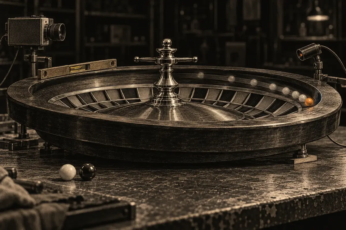
ꯀꯝꯄꯦꯅꯤ ꯑꯃꯁꯨꯡ ꯄꯥꯏ
ꯃꯈꯣꯌꯅ ꯊꯕꯛ ꯑꯁꯤꯕꯨ ꯌꯨꯗꯦꯃꯣꯅꯤꯛ ꯑꯦꯟꯇꯔꯞꯔꯥꯏꯖꯦꯁ (Eudaemonic Enterprises) ꯍꯥꯌꯅ ꯀꯧꯈꯤ, ꯋꯥꯈꯂꯅ ꯂꯃꯖꯤꯡꯕ ꯄꯨꯟꯁꯤ ꯑꯃꯒꯤ ꯅꯨꯡꯉꯥꯏꯕꯒꯤꯗꯃꯛ ꯒ꯭ꯔꯤꯛ ꯋꯥꯍꯩ ꯑꯃꯗꯒꯤ꯫ ꯃꯁꯤꯗ ꯊꯕꯛ ꯇꯧꯈꯤꯕ ꯃꯤ ꯈꯨꯗꯤꯡꯃꯛꯇ ꯃꯈꯣꯌꯅ ꯊꯥꯗꯣꯀꯈꯤꯕ ꯄꯨꯡꯒꯤ ꯃꯇꯨꯡ ꯏꯟꯅꯥ ꯃꯊꯪꯗ ꯃꯥꯏꯄꯥꯛꯇꯨꯅ ꯐꯪꯒꯗꯕ ꯁꯦꯜꯗꯒꯤ ꯄꯤꯒꯗꯕꯅꯤ: ꯃꯈꯣꯌꯅ ꯌꯨꯗꯦꯃꯣꯅꯤꯛ ꯄꯥꯏ ꯍꯥꯌꯅ ꯀꯧꯕꯒꯤ ꯁꯔꯨꯛ ꯑꯃꯥ꯫ ꯃꯥꯏꯄꯥꯛꯇꯨꯅ ꯐꯪꯂꯕ ꯁꯦꯜ ꯑꯗꯨꯅ ꯃꯁꯥꯒꯤ ꯃꯑꯣꯡꯗ ꯁꯥꯏꯟꯁ ꯇꯧꯔꯤꯕ ꯃꯔꯨꯄꯁꯤꯡꯒꯤ ꯈꯨꯟꯅꯥꯏ ꯑꯃꯒꯤꯗꯃꯛ ꯁꯦꯜ ꯄꯤꯒꯗꯕꯅꯤ꯫
ꯈꯣꯉꯕꯥꯛꯀꯤ ꯃꯈꯥꯗ ꯀꯝꯞꯌꯨꯇꯔ ꯑꯃꯥ, 1976–1978
Farmer says the first equipment was worn under the arm and a later version fitted inside a shoe. Toe switches supplied timing information, and vibrating signals communicated the prediction. One person measured the ballꯈꯨꯠꯂꯥꯏꯕꯣꯜꯔꯣꯇꯔꯒꯤ ꯃꯥꯌꯣꯛꯇ ꯇ꯭ꯔꯦꯛꯇ ꯊꯥꯗꯣꯛꯄ ꯑꯄꯤꯛꯄ ꯕꯣꯜ꯫ ꯍꯧꯖꯤꯛꯀꯤ ꯕꯣꯜꯁꯤꯡ ꯑꯥꯏꯚꯣꯔꯤꯟ ꯅꯠꯔꯒ ꯇꯦꯐ꯭ꯂꯣꯅꯅ ꯁꯦꯝꯃꯤ, 18–21 mm꯫ꯃꯄꯨꯡ ꯄꯥꯕꯤꯌꯨ → and rotorꯈꯨꯠꯂꯥꯏꯔꯣꯇꯔꯄꯣꯀꯦꯠꯁꯤꯡ ꯄꯨꯔꯛꯄ ꯆꯛꯔꯒꯤ ꯀꯣꯏꯕ ꯁꯔꯨꯛ꯫ꯃꯄꯨꯡ ꯄꯥꯕꯤꯌꯨ →; another placed bets. The method needed enough time between measuring the spin and the close of betting.
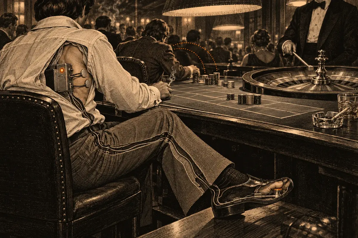
1978ꯒꯤ ꯅꯤꯡꯊꯝ ꯊꯥ
A useful prediction still has to reach the bettor in time. The computer, switches, power supply and communication link all form part of that system. A failure at any stage can make an otherwise useful calculation impossible to act on. This is why a model’s estimated advantage should not be treated as the return of a working casino device.
ꯆꯛꯔꯒꯤ ꯃꯥꯄꯁꯤꯡ ꯑꯃꯁꯨꯡ ꯍꯛꯆꯥꯡꯗ ꯁꯦꯠꯄ ꯌꯥꯕ ꯀꯝꯄꯤꯎꯇꯔ ꯑꯃꯥ, ꯐꯥꯔꯃꯔꯅ ꯐꯣꯡꯗꯣꯀꯈꯤꯕ꯫
ꯔꯦꯗꯤꯑꯣꯒꯤ ꯏꯟꯇꯔꯐꯤꯌꯔꯦꯟꯁꯅ ꯁꯟꯗꯥꯟꯁꯇ ꯇꯧꯈꯤꯕ ꯆꯥꯡꯌꯦꯡ ꯑꯗꯨ ꯁꯣꯀꯍꯅꯈꯤ ꯍꯥꯌꯅ ꯃ꯭ꯌꯨꯖꯤꯌꯃꯅ ꯐꯣꯡꯗꯣꯛꯂꯤ꯫
ꯊꯣꯃꯁ ꯕꯥꯁꯀꯤ The Eudaemonic Pie ꯐꯣꯡꯗꯣꯀꯈꯤ꯫
ꯈꯣꯡꯎꯄꯇ ꯂꯩꯕ ꯀꯝꯞꯌꯨꯇꯔ, 1980–1981
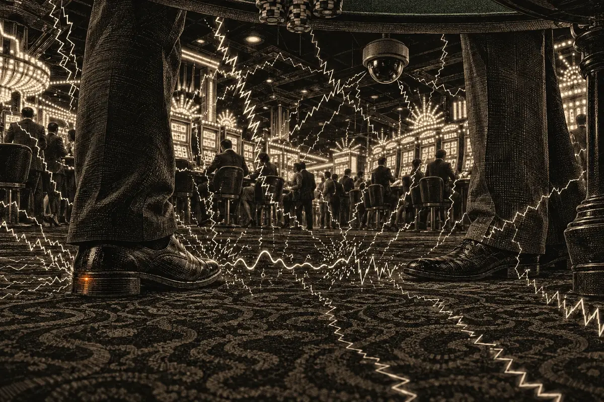
The Heinz Nixdorf MuseumsForum, which displays the shoe computer, describes a November 1981 trial at the Sundance in Las Vegas. Farmer used a toe switch to time the ball. A transmitter sent the predicted wheel sectorꯆꯛꯔꯁꯦꯛꯇꯔꯆꯛꯔꯗ ꯃꯔꯛ ꯂꯩꯇꯅ ꯃꯈꯥ ꯆꯠꯅꯅ ꯂꯩꯕ ꯄꯣꯀꯦꯠꯁꯤꯡꯒꯤ ꯁꯔꯨꯛ, ꯂꯦꯑꯥꯎꯠꯇ ꯂꯩꯕ ꯀꯥꯡꯂꯨꯞ ꯑꯃꯗꯒꯤ ꯇꯣꯉꯥꯟꯅ꯫ꯃꯄꯨꯡ ꯄꯥꯕꯤꯌꯨ → to Bass, who received vibrating signals in his shoe and placed the bets.
The museum reports that casino electronics disrupted the radio link and made the signals unreadable. The team decided against another lengthy rebuild. Its account supports a hardware problem during that trial, not a general claim that electronic prediction always succeeds or always fails.
44% ꯍꯥꯌꯕꯁꯤ ꯀꯔꯤꯅꯣ
On a uniform American wheel, a fixed straight-up bet wins with probabilityꯃꯦꯊꯃꯦꯇꯤꯛꯁꯊꯣꯛꯄꯒꯤ ꯈꯨꯗꯣꯡꯆꯥꯕꯃꯍꯩ ꯑꯃꯥ ꯊꯣꯛꯄꯒꯤ ꯈꯨꯗꯣꯡꯆꯥꯕ, 0 ꯗꯒꯤ 1 ꯐꯥꯑꯣꯕ ꯅꯠꯔꯒ 0% ꯗꯒꯤ 100% ꯐꯥꯑꯣꯕ꯫ ꯃꯁꯤꯡ ꯑꯃꯥ: 1/37 = 2.70%꯫ꯃꯄꯨꯡ ꯄꯥꯕꯤꯌꯨ → 1/38. At a 35:1 net payoutꯁꯦꯜꯄꯦꯑꯥꯎꯠꯃꯥꯏꯄꯥꯛꯄ ꯕꯦꯠ ꯑꯃꯅ ꯍꯜꯂꯛꯄ ꯁꯦꯜ, ꯍꯜꯂꯀꯄ ꯊꯝꯂꯕ ꯁꯦꯜꯒꯤ ꯃꯊꯛꯇ “X ꯗꯒꯤ 1” ꯍꯥꯌꯅ ꯍꯥꯌꯏ꯫ꯃꯄꯨꯡ ꯄꯥꯕꯤꯌꯨ →, its expected return is 36/38 − 1, or −5.26%. If a prediction method truly raises the hit probability to 1/25 on the bets selected, the same calculation gives +44%.
This is conditional arithmetic, not a measurement of the Eudaemons’ device. A real estimate would need the bets placed, the outcomes and uncertainty. Predicting a sector also differs from making a single-number bet; the return must be calculated across the full stake.
ꯑꯆꯧꯕ ꯑꯦꯖ ꯑꯃꯁꯨ ꯀꯔꯤꯒꯤ ꯖꯨꯌꯥꯒꯨꯝ ꯐꯥꯎꯈꯤꯕꯒꯦ
A positive expected return does not make a short session predictable. In an illustrative model with independent spinsꯃꯦꯊꯃꯦꯇꯤꯛꯁꯃꯔꯤ ꯂꯩꯅꯗꯕ ꯁ꯭ꯄꯤꯟꯁꯤꯡꯍꯥꯟꯅꯒꯤ ꯃꯍꯩ ꯀꯔꯤꯒꯨꯝꯕ ꯑꯣꯏꯔꯕꯁꯨ ꯁ꯭ꯄꯤꯟ ꯈꯨꯗꯤꯡꯃꯛꯀꯤ ꯊꯣꯛꯄꯒꯤ ꯈꯨꯗꯣꯡꯆꯥꯕ ꯃꯥꯟꯅꯩ꯫ ꯋꯦꯕꯁꯥꯏꯠ ꯑꯁꯤꯒꯤ ꯊꯤꯕ ꯈꯨꯗꯤꯡꯃꯛꯀꯤ ꯌꯨꯝꯐꯝꯅꯤ꯫ꯃꯄꯨꯡ ꯄꯥꯕꯤꯌꯨ →, one unitꯁꯦꯜꯌꯨꯅꯤꯠꯁꯤꯁ꯭ꯇꯦꯝ ꯅꯠꯔꯒ ꯁꯥꯟꯅꯔꯤꯕ ꯑꯃꯅ ꯁꯤꯖꯤꯟꯅꯕ ꯃꯔꯨꯑꯣꯏꯕ ꯊꯝꯂꯕ ꯁꯦꯜ꯫ ꯄ꯭ꯔꯣꯒ꯭ꯔꯦꯁꯅꯁꯤꯡ ꯌꯨꯅꯤꯠꯇ ꯁꯟꯗꯣꯛꯂꯤ, ꯃꯔꯝ ꯑꯗꯨꯅ ꯃꯈꯣꯌ ꯀꯔꯤꯒꯨꯝꯕ ꯇꯦꯕꯜꯗ ꯆꯠꯂꯤ꯫ꯃꯄꯨꯡ ꯄꯥꯕꯤꯌꯨ → on a single number each spin, a true hit probability of 1/25 and a 35:1 payout, the player is still behind after 100 spins about 23.2% of the time. That is the probability of zeroꯆꯛꯔꯖꯤꯔꯣꯆꯞ ꯃꯥꯟꯅꯕ, ꯗꯖꯟ ꯅꯠꯔꯒ ꯀꯂꯝ ꯕꯦꯠ ꯑꯃꯠꯇꯅ ꯀꯨꯞꯇꯕ ꯑꯁꯪꯕ ꯄꯣꯀꯦꯠ ꯑꯃꯈꯛꯇ; ꯍꯥꯎꯁ ꯑꯦꯖꯀꯤ ꯍꯧꯔꯀꯐꯝꯅꯤ꯫ ꯑꯇꯣꯞꯄ ꯃꯃꯤꯡ: ꯁꯤꯡꯒꯜ ꯖꯤꯔꯣ, 0꯫ꯃꯄꯨꯡ ꯄꯥꯕꯤꯌꯨ →, one or two wins.
This example is not a reconstruction of the group’s sector bets. Smaller stakes reduce the money exposed, but they do not eliminate losses or establish that a particular bankrollꯁꯦꯜꯕꯦꯡꯀꯔꯣꯜꯁꯥꯟꯅꯅꯕ ꯇꯣꯉꯥꯟꯅ ꯊꯝꯂꯕ ꯁꯦꯜ ꯄꯨꯝꯅꯃꯛ꯫ ꯕꯦꯡꯀꯔꯣꯜ ꯃꯦꯅꯦꯖꯃꯦꯟꯠ ꯍꯥꯌꯕꯁꯤ ꯃꯗꯨꯒꯤ ꯀꯌꯥ ꯕꯦꯠ ꯈꯨꯗꯤꯡꯗ ꯑꯃꯁꯨꯡ ꯁꯦꯁꯟ ꯈꯨꯗꯤꯡꯗ ꯈꯨꯗꯣꯡꯊꯤꯕꯗ ꯊꯃꯒꯗꯒꯦ ꯍꯥꯌꯕ ꯋꯥꯔꯦꯞ ꯂꯧꯕꯅꯤ꯫ꯃꯄꯨꯡ ꯄꯥꯕꯤꯌꯨ → is safe.
ꯀꯌꯥ ꯆꯪꯈꯤ ꯑꯃꯁꯨꯡ ꯀꯌꯥ ꯐꯪꯈꯤ
Bass’s preview gives a 44% advantage estimate; Farmer’s retrospective account reports 20%. These figures should stay attached to their sources. Without matching test conditions and betting records, they are not interchangeable measurements.
A percentage advantage is also different from money earned. Net profit would need to account for stakes, payouts, equipment and other costs. The sources used here do not establish a complete audited profit-and-loss account.
ꯍꯧꯖꯤꯛ ꯂꯥꯏꯔꯤꯛ ꯑꯗꯨ ꯄꯥꯕ
ꯑꯔꯣꯏꯕ ꯈꯣꯉꯆꯇꯇ ꯕꯦꯠ ꯊꯃꯈꯤꯕ ꯊꯣꯃꯁ ꯕꯥꯁ (Thomas Bass)ꯅ ꯒ꯭ꯔꯨꯞ ꯑꯗꯨꯒꯥ ꯁꯥꯡꯅ ꯋꯥꯔꯤ ꯁꯥꯅꯈꯤꯕꯗ ꯌꯨꯝꯐꯝ ꯑꯣꯏꯗꯨꯅ The Eudaemonic Pie (1985)ꯗ ꯋꯥꯔꯤ ꯑꯁꯤ ꯇꯥꯀꯈꯤ, ꯑꯃꯁꯨꯡ ꯃꯁꯤ ꯂꯃꯥꯏ ꯑꯁꯤꯒꯤ ꯍꯧꯔꯛꯐꯃꯅꯤ꯫ ꯃꯁꯤꯒꯤ ꯔꯨꯂꯦꯠꯀꯤ ꯊꯨꯅ ꯄꯨꯋꯥꯔꯤ ꯑꯗꯨ ꯄ꯭ꯔꯣꯖꯦꯛꯠꯀꯤ ꯋꯥꯔꯤꯗꯒꯤ ꯊꯥꯖꯕ ꯌꯥꯕ ꯍꯟꯊꯩ꯫ ꯃꯁꯤꯅ ꯖꯦꯒꯔꯅ ꯂꯧꯈꯤꯕ ꯀ꯭ꯂꯥꯔꯛ ꯇꯔꯨꯛꯀꯤ ꯋꯥꯔꯤ ꯑꯃꯨꯛ ꯍꯟꯅꯥ ꯍꯥꯌꯔꯤ, ꯃꯁꯤ 1901ꯒꯤ ꯂꯥꯏꯔꯤꯛ ꯑꯃꯗꯒꯤ ꯍꯦꯟꯅꯥ ꯃꯃꯥꯡꯗ ꯆꯠꯂꯣꯏ (ꯖꯣꯁꯦꯐ ꯖꯦꯒꯔ ꯌꯦꯡꯕꯤꯌꯨ), ꯑꯃꯁꯨꯡ ꯊꯣꯔꯞ ꯑꯃꯁꯨꯡ ꯁꯦꯅꯟꯒꯤ ꯀꯦꯁꯤꯅꯣ ꯇꯦꯁ꯭ꯠ ꯑꯗꯨ 1962ꯗ ꯊꯝꯂꯤ, ꯊꯣꯔꯄꯀꯤ ꯃꯁꯥꯒꯤ ꯋꯥꯔꯤꯁꯤꯡꯅꯗꯤ 1961ꯒꯤ ꯅꯤꯡꯊꯝ ꯊꯥꯅꯤ ꯍꯥꯌꯔꯤ꯫
ꯋꯥꯍꯪꯁꯤꯡ
ꯂꯩꯔꯀꯈꯤꯗꯦ꯫ ꯃꯈꯣꯌꯅ ꯗꯥꯏꯝ ꯑꯃꯁꯨꯡ ꯀ꯭ꯕꯥꯔꯇꯔꯒꯤ ꯊꯝꯂꯕ ꯁꯦꯜꯗ ꯗꯣꯂꯥꯔ ꯂꯤꯁꯤꯡ ꯈꯔꯈꯛ ꯃꯥꯏꯄꯥꯛꯈꯤ, ꯑꯃꯁꯨꯡ $15,000 ꯃꯇꯧ ꯑꯃꯁꯨꯡ ꯄꯨꯡ ꯂꯤꯁꯤꯡ ꯀꯌꯥ ꯆꯪꯈꯤ꯫
ꯃꯈꯣꯌꯅ ꯁꯥꯟꯔꯤꯉꯩꯗ, ꯅꯦꯚꯥꯗꯥꯗ ꯈꯨꯠꯂꯥꯏ ꯑꯃꯅ ꯁꯥꯟꯅꯕ ꯑꯃꯥ ꯂꯥꯎꯊꯣꯀꯄꯒꯤ ꯃꯥꯌꯣꯛꯇ ꯑꯥꯏꯟ ꯂꯩꯈꯤꯗꯦ꯫ 1985ꯗꯒꯤ ꯍꯧꯔꯒꯥ ꯑꯥꯏꯟ ꯑꯃꯥ ꯂꯩꯔꯦ, ꯑꯃꯁꯨꯡ ꯀꯦꯁꯤꯅꯣ ꯂꯩꯕ ꯃꯐꯝ ꯌꯥꯝꯅꯥ ꯀꯌꯥꯗꯁꯨ ꯍꯧꯖꯤꯛ ꯂꯩꯔꯦ꯫
ꯂꯥꯏꯕ ꯁ꯭ꯇꯨꯗꯤꯑꯣꯁꯤꯡꯗ ꯇꯧꯔꯤꯕꯒꯨꯝꯅ ꯕꯣꯜ ꯊꯥꯗꯣꯛꯄꯒꯥ ꯂꯣꯌꯅꯅ ꯕꯦꯠ ꯊꯝꯕ ꯂꯣꯏꯔꯕ ꯃꯐꯃꯗꯗꯤ ꯇꯧꯔꯣꯏ, ꯑꯃꯁꯨꯡ ꯑꯁꯤꯒꯨꯝꯕ ꯈꯨꯠꯂꯥꯏ ꯑꯃꯥ ꯀꯦꯁꯤꯅꯣꯗ ꯄꯨꯔꯛꯄ ꯑꯁꯤ ꯃꯐꯝ ꯌꯥꯝꯅꯥ ꯀꯌꯥꯗ ꯀ꯭ꯔꯥꯏꯝꯅꯤ꯫
ꯃꯦꯊꯃꯦꯇꯤꯛꯁꯀꯥ ꯁꯥꯟꯅꯕ
ꯃꯁꯤꯁꯤꯡ ꯑꯍꯥꯅꯕꯗ ꯅꯍꯥꯛ ꯃꯁꯥꯃꯛꯅ ꯍꯣꯠꯅꯕꯤꯌꯨ꯫ ꯄꯥꯎꯈꯨꯝ ꯈꯨꯗꯤꯡꯃꯛ ꯊꯨꯡꯗꯨꯅ ꯊꯝꯂꯤ; ꯁꯦꯝ ꯁꯥꯔꯕ ꯃꯇꯃꯗ ꯍꯥꯡꯗꯣꯛꯄꯤꯌꯨ꯫
Suppose a prediction gives a straight-up bet paying 35:1 an expected return of +44% of its stake. What hit probabilityꯃꯦꯊꯃꯦꯇꯤꯛꯁꯊꯣꯛꯄꯒꯤ ꯈꯨꯗꯣꯡꯆꯥꯕꯃꯍꯩ ꯑꯃꯥ ꯊꯣꯛꯄꯒꯤ ꯈꯨꯗꯣꯡꯆꯥꯕ, 0 ꯗꯒꯤ 1 ꯐꯥꯑꯣꯕ ꯅꯠꯔꯒ 0% ꯗꯒꯤ 100% ꯐꯥꯑꯣꯕ꯫ ꯃꯁꯤꯡ ꯑꯃꯥ: 1/37 = 2.70%꯫ꯃꯄꯨꯡ ꯄꯥꯕꯤꯌꯨ → does that require? On a 38-pocketꯈꯨꯠꯂꯥꯏꯄꯣꯀꯦꯠꯔꯣꯇꯔꯗ ꯂꯩꯕ ꯃꯁꯤꯡ ꯏꯔꯕ ꯀꯣꯠ 37 ꯒꯤ ꯃꯅꯨꯡꯗ ꯑꯃꯥ꯫ ꯑꯇꯣꯞꯄ ꯃꯃꯤꯡ: ꯁ꯭ꯂꯣꯠ, ꯀꯞ꯫ꯃꯄꯨꯡ ꯄꯥꯕꯤꯌꯨ → wheel, how many pockets would need to be excluded in a model that assigns equal probability to every remaining pocket?
ꯄꯥꯎꯈꯨꯝ ꯎꯠꯄ
ꯄꯥꯎꯈꯨꯝ ꯁ꯭ꯄꯤꯟ 25 ꯗ ꯑꯃꯨꯛ꯫ ꯃꯁꯤ ꯄꯣꯀꯦꯠ 13 ꯊꯥꯗꯣꯛꯇꯨꯅ 25 ꯊꯃꯖꯤꯟꯕꯒꯥ ꯃꯥꯟꯅꯩ꯫
A winning chipꯁꯦꯜꯆꯤꯞꯂꯦꯞꯂꯕ ꯁꯦꯜꯒꯤ ꯃꯃꯜ ꯇꯥꯛꯄ ꯇꯣꯀꯟ, ꯕꯦꯠ ꯊꯝꯅꯕ ꯂꯦꯑꯥꯎꯠꯇ ꯊꯝꯃꯤ꯫ ꯑꯇꯣꯞꯄ ꯃꯃꯤꯡ: ꯆꯦꯛ꯫ꯃꯄꯨꯡ ꯄꯥꯕꯤꯌꯨ → comes back with 35 more: 36 chips. If the number wins once in n spins, n chips staked bring 36 back, so the bet is worth 36/n − 1.
Set that to 0.44: 36/n = 1.44, so n = 25. With no prediction n is 38 and the bet is worth 36/38 − 1 = −5.26%.
Now suppose a prediction rules out k pockets and the ballꯈꯨꯠꯂꯥꯏꯕꯣꯜꯔꯣꯇꯔꯒꯤ ꯃꯥꯌꯣꯛꯇ ꯇ꯭ꯔꯦꯛꯇ ꯊꯥꯗꯣꯛꯄ ꯑꯄꯤꯛꯄ ꯕꯣꯜ꯫ ꯍꯧꯖꯤꯛꯀꯤ ꯕꯣꯜꯁꯤꯡ ꯑꯥꯏꯚꯣꯔꯤꯟ ꯅꯠꯔꯒ ꯇꯦꯐ꯭ꯂꯣꯅꯅ ꯁꯦꯝꯃꯤ, 18–21 mm꯫ꯃꯄꯨꯡ ꯄꯥꯕꯤꯌꯨ → is equally likely to land in each of the other 38 − k. A chip on one of those wins once in 38 − k spins. For 44% we need 38 − k = 25, so k = 13: a little more than a third of the wheel.
This equivalence depends on equal probabilities across the remaining pockets. Excluding eight of 38 pockets gives 36/30 − 1 = +20% in this model. Different probability distributions require their own calculation; this exercise does not measure a historical team’s performance.
ꯊꯥꯗꯣꯀꯈꯤꯕ ꯄꯣꯀꯦꯠꯂꯦꯃꯍꯧꯔꯤꯕ ꯄꯣꯀꯦꯠꯁ꯭ꯇ꯭ꯔꯦꯠ-ꯑꯄꯀꯤ ꯃꯃꯜ038−5.26%2360%830+20%1325+44%1919+89%ꯅꯍꯥꯛꯀꯤ ꯃꯁꯤꯡ ꯑꯗꯨ ꯑꯁꯦꯡꯕꯗ 35 ꯗꯒꯤ 1 ꯗ ꯁ꯭ꯄꯤꯟ 25 ꯗ ꯑꯃꯨꯛ ꯃꯥꯏꯄꯥꯀꯏ ꯍꯥꯌꯅ ꯈꯟꯊꯕꯤꯌꯨ, 44% ꯒꯤ ꯑꯦꯖ꯫ ꯅꯍꯥꯛꯅ ꯁ꯭ꯄꯤꯟ ꯈꯨꯗꯤꯡꯗ ꯆꯤꯞ ꯑꯃꯥ ꯊꯝꯏ꯫ ꯁ꯭ꯄꯤꯟ 100 ꯒꯤ ꯃꯇꯨꯡꯗ ꯃꯥꯡꯈꯤꯕꯗ ꯂꯩꯕꯒꯤ ꯈꯨꯗꯣꯡꯆꯥꯕ ꯀꯌꯥ? 500 ꯒꯤ ꯃꯇꯨꯡꯗ?
ꯄꯥꯎꯈꯨꯝ ꯎꯠꯄ
ꯄꯥꯎꯈꯨꯝ ꯁ꯭ꯄꯤꯟ 100 ꯒꯤ ꯃꯇꯨꯡꯗ 23% ꯈꯔ ꯑꯃꯁꯨꯡ 500 ꯒꯤ ꯃꯇꯨꯡꯗꯁꯨ 6% ꯈꯔ꯫
After 100 spins you have staked 100 chips, and each win brings back 36. Two wins bring 72, a loss of 28; three bring 108, a gain of 8. So you are behind if you win twice or less.
The chance of no win in 100 spins is (24/25)¹⁰⁰ = 1.7%. Exactly one win: 100 × (1/25) × (24/25)⁹⁹ = 7.0%. Exactly two: 4,950 × (1/25)² × (24/25)⁹⁸ = 14.5%. Together 23.2%.
After 500 spins you need 14 wins to be ahead (14 × 36 = 504), and the average is 20. The chance of 13 or fewer is about 6.2%.
A positive expected return can coexist with a substantial chance of finishing behind. These binomial results assume independent spinsꯃꯦꯊꯃꯦꯇꯤꯛꯁꯃꯔꯤ ꯂꯩꯅꯗꯕ ꯁ꯭ꯄꯤꯟꯁꯤꯡꯍꯥꯟꯅꯒꯤ ꯃꯍꯩ ꯀꯔꯤꯒꯨꯝꯕ ꯑꯣꯏꯔꯕꯁꯨ ꯁ꯭ꯄꯤꯟ ꯈꯨꯗꯤꯡꯃꯛꯀꯤ ꯊꯣꯛꯄꯒꯤ ꯈꯨꯗꯣꯡꯆꯥꯕ ꯃꯥꯟꯅꯩ꯫ ꯋꯦꯕꯁꯥꯏꯠ ꯑꯁꯤꯒꯤ ꯊꯤꯕ ꯈꯨꯗꯤꯡꯃꯛꯀꯤ ꯌꯨꯝꯐꯝꯅꯤ꯫ꯃꯄꯨꯡ ꯄꯥꯕꯤꯌꯨ →, a stable hit probability of 1/25, and enough funds to place every planned bet. They do not establish that a real prediction has that accuracy.
ꯁ꯭ꯄꯤꯟꯀꯥꯟꯅꯕꯗ ꯂꯩꯅꯕ ꯃꯊꯧ ꯇꯥꯕ ꯃꯥꯏꯄꯥꯛꯄꯃꯥꯡꯈꯤꯕꯗ ꯂꯩꯕꯒꯤ ꯈꯨꯗꯣꯡꯆꯥꯕ50240.0%100323.2%200618.6%500146.2%ꯂꯥꯏꯔꯤꯛ ꯑꯗꯨꯅ 44% ꯒꯤ ꯑꯦꯖꯒꯥ ꯂꯣꯌꯅꯅ, ꯄꯨꯡ ꯈꯨꯗꯤꯡꯗ ꯑꯃꯨꯛ 50 $100 ꯊꯝꯂꯕꯗꯤ ꯄꯨꯡ ꯈꯨꯗꯤꯡꯗ $2,200 ꯐꯪꯒꯗꯕꯅꯤ ꯍꯥꯌꯔꯤ꯫ ꯃꯁꯤ ꯌꯦꯡꯁꯤꯟꯕꯤꯌꯨ꯫ ꯃꯗꯨꯒꯤ ꯃꯇꯨꯡꯗ ꯀꯥꯡꯂꯨꯞ ꯑꯗꯨꯅ ꯑꯁꯦꯡꯕꯗ ꯁꯥꯟꯅꯈꯤꯕ ꯊꯝꯂꯕ ꯁꯦꯜꯗ ꯑꯦꯖ ꯑꯗꯨꯃꯛꯅ ꯀꯌꯥ ꯐꯪꯈꯤꯕꯒꯦ ꯍꯥꯌꯕ ꯊꯤꯕꯤꯌꯨ: ꯁ꯭ꯄꯤꯟ ꯈꯨꯗꯤꯡꯗ ꯗꯥꯏꯝ ꯑꯃꯥ꯫
ꯄꯥꯎꯈꯨꯝ ꯎꯠꯄ
ꯄꯥꯎꯈꯨꯝ +$2,200 at $100 per bet; +$2.20 at $0.10 per bet; +$8.80 with four $0.10 bets per spin. These are expectations, not hourly guarantees.
Expected profit is the amount staked multiplied by the player edge. At $100 per spin and 50 spins an hour, turnoverꯁꯦꯜꯇꯔꯅꯑꯣꯚꯔꯁꯦꯁꯟ ꯅꯠꯔꯒ ꯃꯇꯝ ꯑꯃꯒꯤ ꯃꯅꯨꯡꯗ ꯕꯦꯠ ꯊꯝꯂꯕ ꯁꯦꯜ ꯄꯨꯝꯅꯃꯛ, ꯑꯃꯨꯛ ꯍꯟꯅꯥ ꯊꯝꯂꯕ ꯃꯥꯏꯄꯥꯛꯇꯨꯅ ꯐꯪꯂꯕ ꯁꯦꯜꯁꯨ ꯌꯥꯎꯅ꯫ ꯑꯇꯣꯞꯄ ꯃꯃꯤꯡ: ꯍꯦꯟꯗꯜ, ꯑꯦꯛꯁꯟ꯫ꯃꯄꯨꯡ ꯄꯥꯕꯤꯌꯨ → is $5,000 and expected profit is $5,000 × 0.44 = $2,200.
At $0.10 per spin, hourly turnover is $5 and the expectation is $2.20. Four $0.10 bets per spin make turnover $20 and expectation $8.80, provided each bet really retains the assumed 44% edge.
The arithmetic scales with stakes. It does not establish a real-world edge or describe the stakes, earnings or motives of a historical group.
ꯅꯣꯛꯅꯕꯒꯤ ꯀꯃꯤꯛ
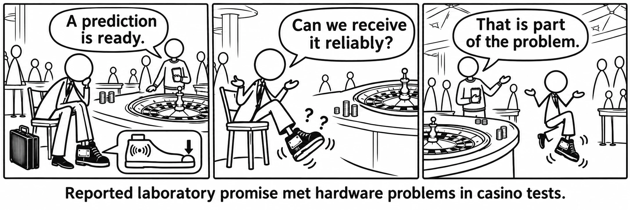
ꯐꯤꯖꯤꯛꯁꯅ ꯊꯕꯛ ꯇꯧꯈꯤ꯫ ꯅꯤꯌꯣꯅꯅ ꯃꯥꯏꯄꯥꯛꯈꯤ꯫
ꯍꯧꯔꯛꯐꯃꯁꯤꯡ
- Bass, T. A. The Eudaemonic Pie.
- Thorp, E. O. “Optimal gambling systems for favorable games.”
- Thorp, E. O. “The invention of the first wearable computer.”
- Nevada Revised Statutes, chapter 465.
- Nevada NRS 465.075 — ꯍꯧꯖꯤꯛꯀꯤ ꯋꯥꯐꯝ 2026ꯒꯤ ꯅꯣꯚꯦꯝꯕꯔ 15ꯗ ꯌꯦꯡꯁꯤꯟꯈꯤ
- Heinz Nixdorf MuseumsForum, Shoe computer — Sundance ꯒꯤ ꯋꯥꯌꯦꯜ
- J. Doyne Farmer, Roulette — ꯌꯥꯎꯈꯤꯕ ꯃꯤꯑꯣꯏ ꯑꯃꯒꯤ ꯋꯥꯔꯤ
- Thomas Bass, The Eudaemonic Pie — ꯄꯥꯕ꯭ꯂꯤꯛ ꯄ꯭ꯔꯤꯚꯤꯌꯨ