ꯁꯦꯝꯄꯜ ꯁꯥꯏꯖ
ꯄꯦꯇꯔꯟ ꯑꯃꯅ ꯑꯔꯊ ꯑꯃꯠꯇꯥ ꯄꯤꯕꯒꯤ ꯃꯃꯥꯡꯗ ꯁ꯭ꯄꯤꯟ ꯀꯌꯥ ꯃꯊꯧ ꯇꯥꯕꯒꯦ꯫

ꯄꯣꯀꯦꯠ ꯑꯃꯅ 37 ꯗꯒꯤ 1 ꯅꯠꯇꯅ 30 ꯗꯒꯤ 1 ꯊꯣꯀꯄꯥ ꯑꯗꯨ ꯆꯨꯝꯅ ꯊꯥꯖꯕ ꯌꯥꯕ ꯃꯑꯣꯡꯗ ꯊꯤꯗꯣꯛꯅꯕꯒꯤꯗꯃꯛ ꯈꯟꯅꯕꯗ ꯁ꯭ꯄꯤꯟ 4,400 ꯃꯊꯧ ꯇꯥꯏ꯫ 35 ꯗꯒꯤ 1 ꯊꯣꯀꯄ ꯄꯣꯀꯦꯠ, ꯇꯁꯦꯡꯅ ꯁꯦꯜ ꯄꯤꯕ ꯌꯥꯕ ꯃꯈꯜ ꯑꯗꯨꯒꯤꯗꯃꯛꯇꯗꯤ ꯁ꯭ꯄꯤꯟ 70,000 ꯈꯟꯅꯕ ꯃꯊꯧ ꯇꯥꯏ꯫
ꯀꯔꯤꯒꯤ ꯃꯁꯤꯡ ꯑꯁꯨꯛ ꯌꯥꯝꯅ ꯃꯊꯧ ꯇꯥꯕꯒꯦ
For n independent spinsꯃꯦꯊꯃꯦꯇꯤꯛꯁꯃꯔꯤ ꯂꯩꯅꯗꯕ ꯁ꯭ꯄꯤꯟꯁꯤꯡꯍꯥꯟꯅꯒꯤ ꯃꯍꯩ ꯀꯔꯤꯒꯨꯝꯕ ꯑꯣꯏꯔꯕꯁꯨ ꯁ꯭ꯄꯤꯟ ꯈꯨꯗꯤꯡꯃꯛꯀꯤ ꯊꯣꯛꯄꯒꯤ ꯈꯨꯗꯣꯡꯆꯥꯕ ꯃꯥꯟꯅꯩ꯫ ꯋꯦꯕꯁꯥꯏꯠ ꯑꯁꯤꯒꯤ ꯊꯤꯕ ꯈꯨꯗꯤꯡꯃꯛꯀꯤ ꯌꯨꯝꯐꯝꯅꯤ꯫ꯃꯄꯨꯡ ꯄꯥꯕꯤꯌꯨ →, the hit count has standard deviationꯃꯦꯊꯃꯦꯇꯤꯛꯁꯁ꯭ꯇꯦꯟꯗꯔꯗ ꯗꯤꯚꯤꯌꯦꯁꯟꯚꯦꯌꯔꯤꯌꯦꯟꯁꯀꯤ ꯁ꯭ꯀ꯭ꯋꯦꯌꯔ ꯔꯨꯠ; ꯃꯍꯩ ꯑꯃꯅ ꯐꯪꯒꯗꯕ ꯃꯃꯜꯗꯒꯤ ꯌꯥꯝꯅ ꯂꯥꯞꯄ ꯃꯑꯣꯡ꯫ꯃꯄꯨꯡ ꯄꯥꯕꯤꯌꯨ → √(np(1−p)); the estimated hit rate has standard error √(p(1−p)/n). Counts get noisier in absolute terms as n grows, while the uncertainty in the rate shrinks. Halving that rate uncertainty requires about four times as many spins.
ꯐꯣꯔꯃꯨꯂꯥ
For a one-sided test of a single pocketꯈꯨꯠꯂꯥꯏꯄꯣꯀꯦꯠꯔꯣꯇꯔꯗ ꯂꯩꯕ ꯃꯁꯤꯡ ꯏꯔꯕ ꯀꯣꯠ 37 ꯒꯤ ꯃꯅꯨꯡꯗ ꯑꯃꯥ꯫ ꯑꯇꯣꯞꯄ ꯃꯃꯤꯡ: ꯁ꯭ꯂꯣꯠ, ꯀꯞ꯫ꯃꯄꯨꯡ ꯄꯥꯕꯤꯌꯨ → at the 5% level with 80% power, the required n is approximately ((1.645·√(p₀(1−p₀)) + 0.84·√(p₁(1−p₁))) / (p₁ − p₀))², with p₀ = 1/37 and p₁ the suspected rate. That holds for one pocket chosen in advance. Searching all 37 pockets requires a multiple-testing design; there is no universal sample-size multiplier. This tests departure from 1/37, not a profitable rate above 1/36.
ꯊꯕꯛꯇ ꯀꯔꯝꯅ ꯄꯥꯕꯒꯦ
Sample size alone does not make an observation evidence or noise. Specify the effect, test and error rates before collecting data. A small sample can identify an extreme failure, while even a large sample may miss a very small departure. Replication and reliable recording remain necessary.
ꯗꯦꯇꯥꯒꯤ ꯃꯃꯜ
At 50 spins an hour, recording 10,000 rounds takes 200 hours. Equipment changes during that time can complicate interpretation. That practical constraint does not establish that all bias detection is impossible or that every historical investigation took months.
ꯍꯥꯎꯁ ꯑꯦꯖ ꯃꯁꯥꯒꯤ ꯁꯦꯝꯄꯜ ꯁꯥꯏꯖ
For a unitꯁꯦꯜꯌꯨꯅꯤꯠꯁꯤꯁ꯭ꯇꯦꯝ ꯅꯠꯔꯒ ꯁꯥꯟꯅꯔꯤꯕ ꯑꯃꯅ ꯁꯤꯖꯤꯟꯅꯕ ꯃꯔꯨꯑꯣꯏꯕ ꯊꯝꯂꯕ ꯁꯦꯜ꯫ ꯄ꯭ꯔꯣꯒ꯭ꯔꯦꯁꯅꯁꯤꯡ ꯌꯨꯅꯤꯠꯇ ꯁꯟꯗꯣꯛꯂꯤ, ꯃꯔꯝ ꯑꯗꯨꯅ ꯃꯈꯣꯌ ꯀꯔꯤꯒꯨꯝꯕ ꯇꯦꯕꯜꯗ ꯆꯠꯂꯤ꯫ꯃꯄꯨꯡ ꯄꯥꯕꯤꯌꯨ → even-money single-zeroꯆꯛꯔꯖꯤꯔꯣꯆꯞ ꯃꯥꯟꯅꯕ, ꯗꯖꯟ ꯅꯠꯔꯒ ꯀꯂꯝ ꯕꯦꯠ ꯑꯃꯠꯇꯅ ꯀꯨꯞꯇꯕ ꯑꯁꯪꯕ ꯄꯣꯀꯦꯠ ꯑꯃꯈꯛꯇ; ꯍꯥꯎꯁ ꯑꯦꯖꯀꯤ ꯍꯧꯔꯀꯐꯝꯅꯤ꯫ ꯑꯇꯣꯞꯄ ꯃꯃꯤꯡ: ꯁꯤꯡꯒꯜ ꯖꯤꯔꯣ, 0꯫ꯃꯄꯨꯡ ꯄꯥꯕꯤꯌꯨ → bet, the mean is −1/37 and the standard deviation is √(1368)/37. After 1,368 independent bets, expected lossꯃꯦꯊꯃꯦꯇꯤꯛꯁꯃꯥꯡꯒꯗꯕ ꯁꯦꯜꯐꯪꯒꯗꯕ ꯃꯃꯂꯕꯨ ꯕꯦꯠ ꯊꯝꯂꯕ ꯁꯦꯜ ꯄꯨꯝꯅꯃꯛꯅ ꯃꯅꯥꯡꯕ; ꯁꯦꯁꯟ ꯅꯠꯔꯒ ꯃꯇꯝ ꯑꯃꯒꯤ ꯃꯅꯨꯡꯗ ꯃꯥꯡꯕ ꯑꯦꯚꯔꯦꯖ ꯁꯦꯜ꯫ꯃꯄꯨꯡ ꯄꯥꯕꯤꯌꯨ → is one standard deviation of the total. At 10,000 it is about 2.70 standard deviations. Neither threshold guarantees a losing result or validates a system.
ꯐꯣꯔꯃꯨꯂꯥ
ꯋꯥꯍꯪꯁꯤꯡ
No. Grouping helps only when the alternative concentrates enough extra probabilityꯃꯦꯊꯃꯦꯇꯤꯛꯁꯊꯣꯛꯄꯒꯤ ꯈꯨꯗꯣꯡꯆꯥꯕꯃꯍꯩ ꯑꯃꯥ ꯊꯣꯛꯄꯒꯤ ꯈꯨꯗꯣꯡꯆꯥꯕ, 0 ꯗꯒꯤ 1 ꯐꯥꯑꯣꯕ ꯅꯠꯔꯒ 0% ꯗꯒꯤ 100% ꯐꯥꯑꯣꯕ꯫ ꯃꯁꯤꯡ ꯑꯃꯥ: 1/37 = 2.70%꯫ꯃꯄꯨꯡ ꯄꯥꯕꯤꯌꯨ → in that sectorꯆꯛꯔꯁꯦꯛꯇꯔꯆꯛꯔꯗ ꯃꯔꯛ ꯂꯩꯇꯅ ꯃꯈꯥ ꯆꯠꯅꯅ ꯂꯩꯕ ꯄꯣꯀꯦꯠꯁꯤꯡꯒꯤ ꯁꯔꯨꯛ, ꯂꯦꯑꯥꯎꯠꯇ ꯂꯩꯕ ꯀꯥꯡꯂꯨꯞ ꯑꯃꯗꯒꯤ ꯇꯣꯉꯥꯟꯅ꯫ꯃꯄꯨꯡ ꯄꯥꯕꯤꯌꯨ →. It can dilute a localized pocket effect.
ꯌꯥꯏ, ꯍꯨꯏꯜ ꯍꯦꯗ ꯑꯗꯨ ꯃꯈꯥ ꯆꯠꯊꯕ ꯑꯃꯁꯨꯡ ꯁꯔꯚꯤꯁ ꯇꯧꯗꯕ ꯑꯣꯏꯔꯕꯗꯤ꯫ ꯃꯗꯨ ꯈꯉꯕ ꯑꯁꯤꯅꯤ ꯈ꯭ꯕꯥꯏꯗꯒꯤ ꯀꯠꯊꯣꯛꯄ꯫
ꯆꯠꯅꯕꯤ ꯑꯣꯏꯅꯥ꯫ ꯃꯁꯤꯒꯤ ꯑꯔꯊꯗꯤ ꯍꯥꯌꯔꯕ ꯆꯥꯡ ꯑꯣꯏꯕ ꯑꯁꯦꯡꯕ ꯕꯥꯏꯌꯥꯁ ꯑꯃꯥ ꯑꯃꯨꯛ ꯃꯉꯥꯗꯒꯤ ꯑꯃꯨꯛ ꯃꯔꯤ ꯊꯤꯗꯣꯛꯀꯅꯤ꯫
ꯅꯣꯛꯅꯕꯒꯤ ꯀꯃꯤꯛ
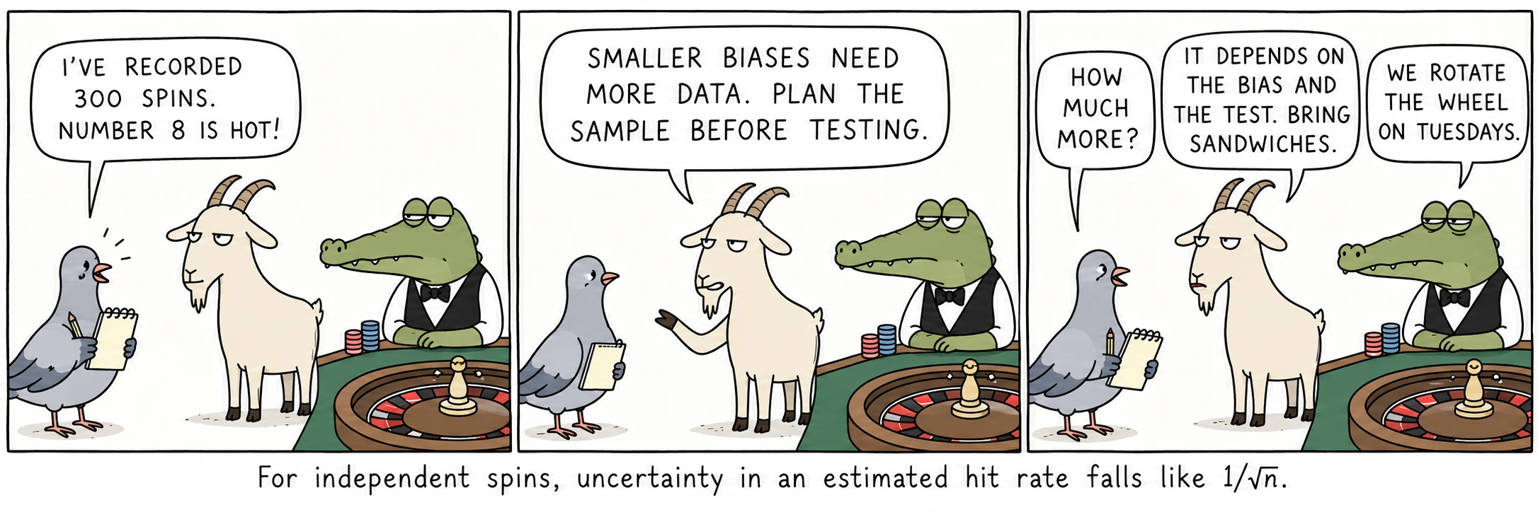
ꯅꯣꯏꯖ 1/√n ꯒꯨꯝꯅ ꯍꯟꯊꯏ꯫ ꯑꯁꯥꯎꯕ ꯊꯤꯡꯕ ꯉꯝꯕ ꯑꯗꯨꯗꯤ ꯍꯦꯟꯅꯥ ꯊꯨꯅꯥ ꯍꯟꯊꯏ꯫
ꯍꯧꯔꯛꯐꯃꯁꯤꯡ
- Feller, W. An Introduction to Probability Theory and Its Applications, Vol. 1.
- Barnhart, R. T. Beating the Wheel.
- ꯁꯦꯝꯄꯜ ꯁꯥꯏꯖꯒꯤ ꯍꯤꯁꯥꯕ