ꯑꯔꯥꯟꯕ ꯊꯥꯖꯕ: ꯃꯇꯝ ꯄꯨꯝꯕꯗ ꯃꯥꯏꯄꯥꯛꯄ ꯔꯨꯂꯦꯠ ꯊꯧꯔꯥꯡ
“ꯑꯩꯒꯤ ꯃꯇꯃꯒꯤ 80% ꯗ ꯃꯥꯏꯄꯥꯀꯄ ꯁꯤꯁ꯭ꯇꯦꯝ ꯑꯃꯥ ꯂꯩ꯫” ꯂꯩꯕ ꯌꯥꯏ꯫ ꯃꯗꯨꯅ ꯍꯧꯖꯤꯛꯁꯨ ꯁꯦꯜ ꯃꯥꯡꯍꯜꯂꯤ꯫

ꯁꯤꯁ꯭ꯇꯦꯝ ꯑꯃꯅ ꯃꯥꯏꯄꯥꯀꯄ ꯁꯦꯁꯟꯁꯤꯡ ꯌꯥꯝꯅ ꯊꯣꯛꯍꯟꯕ ꯉꯝꯃꯤ꯫ ꯐꯪꯒꯗꯕ ꯃꯃꯜ ꯄꯣꯖꯤꯇꯤꯕ ꯑꯣꯏꯍꯟꯕ ꯉꯃꯗꯦ, ꯃꯔꯃꯗꯤ ꯃꯁꯤꯅ ꯊꯝꯕ ꯕꯦꯠ ꯈꯨꯗꯤꯡꯃꯛ ꯃꯁꯥꯒꯤ ꯊꯝꯂꯕ ꯁꯦꯜꯒꯤ −1/37 ꯅꯤ ꯑꯃꯁꯨꯡ ꯐꯪꯒꯗꯕ ꯃꯃꯂꯁꯤꯡ ꯄꯨꯟꯁꯤꯟꯅꯕ ꯌꯥꯏ꯫ ꯈ꯭ꯕꯥꯏꯗꯒꯤ ꯌꯥꯝꯅ ꯃꯥꯏꯄꯥꯀꯄ ꯁꯤꯁ꯭ꯇꯦꯝꯁꯤꯡꯅ ꯃꯥꯏꯊꯤꯕꯗ ꯈ꯭ꯕꯥꯏꯗꯒꯤ ꯌꯥꯝꯅ ꯃꯥꯡꯏ꯫
ꯍꯥꯌꯔꯤꯕ ꯋꯥ
ꯊꯥꯖꯕ ꯑꯗꯨ: ꯀꯗꯥꯏꯗꯃꯛꯇ ꯃꯇꯝ ꯄꯨꯝꯕꯗ ꯃꯥꯏꯄꯥꯀꯄ ꯔꯨꯂꯦꯠ ꯊꯧꯔꯥꯡ ꯑꯃꯥ ꯂꯩ, ꯃꯃꯥꯡꯒꯤ ꯃꯍꯩꯁꯤꯡꯒꯤ ꯃꯇꯨꯡ ꯏꯟꯅ ꯊꯝꯂꯕ ꯁꯦꯜ ꯍꯣꯡꯗꯣꯛꯄ ꯁꯤꯁ꯭ꯇꯦꯝ ꯑꯃꯥ, ꯃꯁꯤꯅ ꯔꯨꯂꯦꯠ ꯑꯁꯤ ꯃꯥꯏꯄꯥꯀꯄ ꯁꯥꯟꯅꯕ ꯑꯃꯗ ꯑꯣꯟꯊꯣꯀꯏ꯫ ꯄꯤꯔꯤꯕ ꯈꯨꯗꯝ: ꯃꯈꯥ ꯇꯥꯅ ꯃꯥꯏꯄꯥꯀꯄ ꯁꯦꯁꯟꯁꯤꯡ, ꯃꯇꯝ ꯈꯨꯗꯤꯡꯗ ꯔꯨꯂꯦꯠꯇ ꯀꯔꯝꯅ ꯃꯥꯏꯄꯥꯛꯀꯗꯒꯦ ꯍꯥꯌꯕꯒꯤ ꯚꯤꯗꯤꯑꯣ ꯑꯃꯥ, ꯁꯥꯛꯁꯤ ꯑꯃꯥ, ꯂꯥꯛ ꯐꯕ ꯍꯞꯇꯥ ꯑꯃꯒꯤ ꯁ꯭ꯞꯔꯦꯗꯁꯤꯠ ꯑꯃꯥ꯫ ꯍꯥꯌꯔꯤꯕ ꯋꯥ ꯑꯁꯤ ꯃꯇꯝ ꯌꯥꯝꯗ ꯊꯥꯖꯕꯥ ꯌꯥꯕꯅꯤ; ꯃꯤ ꯑꯗꯨꯅ ꯃꯁꯤ ꯊꯕꯛ ꯇꯧꯔꯤꯕꯅꯥ ꯊꯥꯖꯩ꯫
ꯀꯔꯤꯒꯤ ꯑꯔꯥꯟꯕꯅꯣ, ꯂꯥꯏꯟ ꯑꯃꯗ
For an independent uniform single-zeroꯆꯛꯔꯖꯤꯔꯣꯆꯞ ꯃꯥꯟꯅꯕ, ꯗꯖꯟ ꯅꯠꯔꯒ ꯀꯂꯝ ꯕꯦꯠ ꯑꯃꯠꯇꯅ ꯀꯨꯞꯇꯕ ꯑꯁꯪꯕ ꯄꯣꯀꯦꯠ ꯑꯃꯈꯛꯇ; ꯍꯥꯎꯁ ꯑꯦꯖꯀꯤ ꯍꯧꯔꯀꯐꯝꯅꯤ꯫ ꯑꯇꯣꯞꯄ ꯃꯃꯤꯡ: ꯁꯤꯡꯒꯜ ꯖꯤꯔꯣ, 0꯫ꯃꯄꯨꯡ ꯄꯥꯕꯤꯌꯨ → model with standard full-loss-on-zero payoutsꯁꯦꯜꯄꯦꯑꯥꯎꯠꯃꯥꯏꯄꯥꯛꯄ ꯕꯦꯠ ꯑꯃꯅ ꯍꯜꯂꯛꯄ ꯁꯦꯜ, ꯍꯜꯂꯀꯄ ꯊꯝꯂꯕ ꯁꯦꯜꯒꯤ ꯃꯊꯛꯇ “X ꯗꯒꯤ 1” ꯍꯥꯌꯅ ꯍꯥꯌꯏ꯫ꯃꯄꯨꯡ ꯄꯥꯕꯤꯌꯨ →, each unitꯁꯦꯜꯌꯨꯅꯤꯠꯁꯤꯁ꯭ꯇꯦꯝ ꯅꯠꯔꯒ ꯁꯥꯟꯅꯔꯤꯕ ꯑꯃꯅ ꯁꯤꯖꯤꯟꯅꯕ ꯃꯔꯨꯑꯣꯏꯕ ꯊꯝꯂꯕ ꯁꯦꯜ꯫ ꯄ꯭ꯔꯣꯒ꯭ꯔꯦꯁꯅꯁꯤꯡ ꯌꯨꯅꯤꯠꯇ ꯁꯟꯗꯣꯛꯂꯤ, ꯃꯔꯝ ꯑꯗꯨꯅ ꯃꯈꯣꯌ ꯀꯔꯤꯒꯨꯝꯕ ꯇꯦꯕꯜꯗ ꯆꯠꯂꯤ꯫ꯃꯄꯨꯡ ꯄꯥꯕꯤꯌꯨ → staked has expected net return −1/37. In a bounded session, with bets chosen using information available before each spin, expected lossꯃꯦꯊꯃꯦꯇꯤꯛꯁꯃꯥꯡꯒꯗꯕ ꯁꯦꯜꯐꯪꯒꯗꯕ ꯃꯃꯂꯕꯨ ꯕꯦꯠ ꯊꯝꯂꯕ ꯁꯦꯜ ꯄꯨꯝꯅꯃꯛꯅ ꯃꯅꯥꯡꯕ; ꯁꯦꯁꯟ ꯅꯠꯔꯒ ꯃꯇꯝ ꯑꯃꯒꯤ ꯃꯅꯨꯡꯗ ꯃꯥꯡꯕ ꯑꯦꯚꯔꯦꯖ ꯁꯦꯜ꯫ꯃꯄꯨꯡ ꯄꯥꯕꯤꯌꯨ → is 1/37 of expected turnoverꯁꯦꯜꯇꯔꯅꯑꯣꯚꯔꯁꯦꯁꯟ ꯅꯠꯔꯒ ꯃꯇꯝ ꯑꯃꯒꯤ ꯃꯅꯨꯡꯗ ꯕꯦꯠ ꯊꯝꯂꯕ ꯁꯦꯜ ꯄꯨꯝꯅꯃꯛ, ꯑꯃꯨꯛ ꯍꯟꯅꯥ ꯊꯝꯂꯕ ꯃꯥꯏꯄꯥꯛꯇꯨꯅ ꯐꯪꯂꯕ ꯁꯦꯜꯁꯨ ꯌꯥꯎꯅ꯫ ꯑꯇꯣꯞꯄ ꯃꯃꯤꯡ: ꯍꯦꯟꯗꯜ, ꯑꯦꯛꯁꯟ꯫ꯃꯄꯨꯡ ꯄꯥꯕꯤꯌꯨ →.
This statement needs its assumptions. Different payouts require a different edge, and an unbounded theoretical stopping rule cannot be handled by silently ignoring convergence conditions. A finite bankrollꯁꯦꯜꯕꯦꯡꯀꯔꯣꯜꯁꯥꯟꯅꯅꯕ ꯇꯣꯉꯥꯟꯅ ꯊꯝꯂꯕ ꯁꯦꯜ ꯄꯨꯝꯅꯃꯛ꯫ ꯕꯦꯡꯀꯔꯣꯜ ꯃꯦꯅꯦꯖꯃꯦꯟꯠ ꯍꯥꯌꯕꯁꯤ ꯃꯗꯨꯒꯤ ꯀꯌꯥ ꯕꯦꯠ ꯈꯨꯗꯤꯡꯗ ꯑꯃꯁꯨꯡ ꯁꯦꯁꯟ ꯈꯨꯗꯤꯡꯗ ꯈꯨꯗꯣꯡꯊꯤꯕꯗ ꯊꯃꯒꯗꯒꯦ ꯍꯥꯌꯕ ꯋꯥꯔꯦꯞ ꯂꯧꯕꯅꯤ꯫ꯃꯄꯨꯡ ꯄꯥꯕꯤꯌꯨ →, table limitsꯇꯦꯕꯜꯇꯦꯕꯜꯒꯤ ꯉꯝꯈꯩꯌꯥꯍꯜꯂꯤꯕ ꯈ꯭ꯕꯥꯏꯗꯒꯤ ꯅꯦꯝꯕ ꯑꯃꯁꯨꯡ ꯈ꯭ꯕꯥꯏꯗꯒꯤ ꯋꯥꯡꯕ ꯕꯦꯠ꯫ ꯈ꯭ꯕꯥꯏꯗꯒꯤ ꯋꯥꯡꯕ ꯉꯝꯈꯩ ꯑꯗꯨꯅ ꯑꯅꯤ ꯊꯥꯛ ꯍꯦꯅꯒꯠꯍꯟꯕ ꯄ꯭ꯔꯣꯒ꯭ꯔꯦꯁꯅꯁꯤꯡ ꯊꯤꯡꯏ꯫ꯃꯄꯨꯡ ꯄꯥꯕꯤꯌꯨ → and a defined stopping rule make a real system concrete enough to evaluate.
ꯀꯔꯤꯒꯤ ꯊꯕꯛ ꯇꯧꯔꯤꯕꯒꯨꯝ ꯎꯕꯒꯦ
Some progressionsꯊꯧꯔꯥꯡꯄ꯭ꯔꯣꯒ꯭ꯔꯦꯁꯟꯃꯃꯥꯡꯒꯤ ꯃꯍꯩꯁꯤꯡꯒꯤ ꯃꯈꯥꯗ ꯊꯝꯂꯕ ꯁꯦꯜ ꯍꯣꯡꯍꯟꯕ ꯅꯤꯌꯝ ꯀꯔꯤꯒꯨꯝꯕ꯫ ꯅꯦꯒꯦꯇꯤꯕ ꯄ꯭ꯔꯣꯒ꯭ꯔꯦꯁꯅꯁꯤꯡꯅ ꯃꯥꯏꯊꯤꯔꯕꯥ ꯃꯇꯨꯡꯗ ꯍꯦꯅꯒꯠꯍꯜꯂꯤ, ꯄꯣꯖꯤꯇꯤꯕꯁꯤꯡꯅ ꯃꯥꯏꯄꯥꯛꯂꯕꯥ ꯃꯇꯨꯡꯗ꯫ꯃꯄꯨꯡ ꯄꯥꯕꯤꯌꯨ → produce frequent small wins and occasional larger losses. The exact frequency depends on the bankroll, maximum stake, session length and reset rules. There is no universal 80% Martingaleꯊꯧꯔꯥꯡꯃꯥꯔꯇꯤꯟꯒꯦꯜꯃꯥꯏꯊꯤꯕ ꯈꯨꯗꯤꯡꯒꯤ ꯃꯇꯨꯡꯗ ꯕꯦꯠ ꯑꯗꯨ ꯑꯅꯤ ꯊꯥꯛ ꯍꯦꯅꯒꯠꯍꯟꯕ ꯄ꯭ꯔꯣꯒ꯭ꯔꯦꯁꯟ꯫ ꯃꯁꯤꯅ ꯀꯔꯤ ꯇꯧꯕꯒꯦ ꯑꯃꯁꯨꯡ ꯀꯔꯤ ꯇꯧꯗꯕꯒꯦ ꯍꯥꯌꯕ ꯊꯧꯔꯥꯡꯒꯤ ꯁꯦꯛꯁꯅꯗ ꯌꯦꯡꯕꯤꯌꯨ꯫ꯃꯄꯨꯡ ꯄꯥꯕꯤꯌꯨ → session-win rate.
For an illustrative comparison, suppose a session wins $40 with probabilityꯃꯦꯊꯃꯦꯇꯤꯛꯁꯊꯣꯛꯄꯒꯤ ꯈꯨꯗꯣꯡꯆꯥꯕꯃꯍꯩ ꯑꯃꯥ ꯊꯣꯛꯄꯒꯤ ꯈꯨꯗꯣꯡꯆꯥꯕ, 0 ꯗꯒꯤ 1 ꯐꯥꯑꯣꯕ ꯅꯠꯔꯒ 0% ꯗꯒꯤ 100% ꯐꯥꯑꯣꯕ꯫ ꯃꯁꯤꯡ ꯑꯃꯥ: 1/37 = 2.70%꯫ꯃꯄꯨꯡ ꯄꯥꯕꯤꯌꯨ → 80% and loses $500 with probability 20%. Its expected result is 0.8 × $40 − 0.2 × $500 = −$68. These assumed outcomes are not simulated results for a particular Martingale configuration.
ꯀꯅꯥꯒꯨꯝꯕ ꯑꯃꯅ ꯇꯧꯕ ꯉꯝꯕ ꯆꯥꯡ ꯌꯦꯡꯕ
The Strategy Simulator can help explore a specified configuration. Read its bankroll, bet rules, session length and stopping conditions before interpreting the output. A finite simulation can have a positive sample mean even when the theoretical expected return is negative. Repeatability and uncertainty matter; neither one winning session nor a simulation alone proves a universal claim.
ꯃꯥꯏꯊꯤꯕ ꯉꯃꯗꯕ ꯁꯤꯁ꯭ꯇꯦꯝ ꯑꯃꯥ
Not placing a wager avoids gambling losses. That is different from finding a betting method with a guaranteed profit. A rule advertised as risk-free may conceal this distinction, an uncovered outcome, a funding requirement or a limit it cannot satisfy.
ꯃꯃꯤꯡ ꯂꯩꯕ ꯁꯤꯁ꯭ꯇꯦꯝꯁꯤꯡ, ꯈꯨꯗꯤꯡꯃꯛ ꯂꯥꯏꯟ ꯑꯃꯗ
ꯃꯃꯤꯡ ꯑꯃꯒ ꯂꯣꯌꯅꯅ, ꯅꯠꯔꯒ ꯔꯨꯂꯦꯠ ꯃꯥꯏꯄꯥꯛꯅꯕꯒꯤ ꯐꯣꯔꯃꯨꯂꯥ ꯑꯣꯏꯅ ꯌꯣꯟꯂꯤꯕ ꯁꯤꯁ꯭ꯇꯦꯝꯁꯤꯡ ꯈꯦꯟꯅꯗꯦ꯫ ꯈꯨꯗꯤꯡꯃꯛ ꯕꯦꯠꯁꯤꯡꯒꯤ ꯁꯦꯠ ꯑꯃꯅꯤ, ꯑꯃꯁꯨꯡ ꯕꯦꯠ ꯈꯨꯗꯤꯡꯅ ꯆꯛꯔꯗ ꯃꯁꯥꯒꯤ 2.70% ꯄꯤ꯫ ꯕꯣꯜꯃꯦꯟ (2024) ꯅ ꯑꯃꯦꯔꯤꯀꯟ ꯆꯛꯔ ꯑꯃꯒꯤꯗꯃꯛ ꯀꯌꯥ ꯍꯤꯁꯥꯕ ꯇꯧꯔꯤ, ꯃꯐꯝ ꯑꯗꯨꯗ ꯈꯨꯗꯤꯡꯃꯛꯅ 5.26% ꯆꯪꯏ; ꯃꯐꯝ ꯑꯁꯤꯗ ꯃꯈꯣꯌ ꯌꯨꯔꯣꯄꯤꯌꯟ ꯆꯛꯔ ꯑꯃꯗ ꯂꯩ꯫
ꯊꯥꯖꯕꯥ ꯌꯥꯕ ꯃꯑꯣꯡ
Stake rules change the distribution of session results and the amount wagered. Under the stated model they do not create an advantage. A progression costs more in expectation than another plan only when it produces more expected turnover at the same house edgeꯃꯦꯊꯃꯦꯇꯤꯛꯁꯍꯥꯎꯁ ꯑꯦꯖꯊꯝꯂꯕ ꯁꯦꯜ ꯈꯨꯗꯤꯡꯗꯒꯤ ꯀꯦꯁꯤꯅꯣꯅ ꯑꯦꯚꯔꯦꯖꯗ ꯊꯃꯖꯤꯜꯂꯤꯕ ꯁꯔꯨꯛ: ꯌꯨꯔꯣꯄꯤꯌꯟ ꯔꯨꯂꯦꯠꯇ 2.70%꯫ꯃꯄꯨꯡ ꯄꯥꯕꯤꯌꯨ →; larger total stakes should not be assumed without comparing the plans.
ꯋꯥꯍꯪꯁꯤꯡ
ꯍꯞꯇꯥ ꯈꯨꯗꯤꯡꯒꯤ ꯁꯦꯁꯟꯒꯤ ꯊꯥ ꯇꯔꯨꯛ ꯍꯥꯌꯕꯁꯤ ꯁꯦꯁꯟ ꯃꯇꯧ ꯀꯨꯞꯅ 25 ꯅꯤ꯫ ꯃꯥꯔꯇꯤꯟꯒꯦꯜꯅ ꯃꯈꯣꯌꯒꯤ 80% ꯃꯥꯏꯄꯥꯀꯏ꯫ ꯃꯥꯏꯊꯤꯕ ꯁꯦꯁꯟꯁꯤꯡ ꯂꯥꯛꯂꯤ, ꯑꯃꯁꯨꯡ ꯃꯈꯣꯌ ꯍꯦꯟꯅꯥ ꯆꯥꯎꯏ꯫
No. A stopping rule changes exposure and the distribution of results. It does not create positive expectation under the stated bounded-session model.
It could change the probability model if supported by evidence. That is different from merely changing stakes after independent results.
ꯃꯦꯊꯃꯦꯇꯤꯛꯁꯀꯥ ꯁꯥꯟꯅꯕ
ꯃꯁꯤꯁꯤꯡ ꯑꯍꯥꯅꯕꯗ ꯅꯍꯥꯛ ꯃꯁꯥꯃꯛꯅ ꯍꯣꯠꯅꯕꯤꯌꯨ꯫ ꯄꯥꯎꯈꯨꯝ ꯈꯨꯗꯤꯡꯃꯛ ꯊꯨꯡꯗꯨꯅ ꯊꯝꯂꯤ; ꯁꯦꯝ ꯁꯥꯔꯕ ꯃꯇꯃꯗ ꯍꯥꯡꯗꯣꯛꯄꯤꯌꯨ꯫
ꯃꯥꯏꯛ ꯀꯦꯔꯣ (Mike Caro) ꯅ 1997 ꯗ ꯑꯃꯦꯔꯤꯀꯟ ꯆꯛꯔꯒꯤꯗꯃꯛ ꯅꯥꯛꯅꯕꯒꯤ ꯑꯣꯏꯅ ꯁꯦꯃꯈꯤꯕ ꯁꯤꯁ꯭ꯇꯦꯝ ꯑꯃꯅ ꯑꯉꯥꯡꯕꯕꯦꯠꯑꯉꯥꯡꯕꯑꯉꯥꯡꯕ ꯃꯁꯤꯡ 18 ꯗ ꯊꯝꯕ ꯆꯞ ꯃꯥꯟꯅꯕ ꯕꯦꯠ꯫ ꯐ꯭ꯔꯦꯟꯆ: ꯔꯨꯖ꯫ꯃꯄꯨꯡ ꯄꯥꯕꯤꯌꯨ → ꯑꯃꯁꯨꯡ ꯑꯃꯨꯕꯕꯦꯠꯑꯃꯨꯕꯑꯃꯨꯕ ꯃꯁꯤꯡ 18 ꯗ ꯊꯝꯕ ꯆꯞ ꯃꯥꯟꯅꯕ ꯕꯦꯠ꯫ ꯐ꯭ꯔꯦꯟꯆ: ꯅꯣꯌꯥꯔ꯫ꯃꯄꯨꯡ ꯄꯥꯕꯤꯌꯨ →, ꯕꯤꯖꯣꯔ ꯑꯃꯁꯨꯡ ꯖꯣꯔ, ꯑꯃꯁꯨꯡ ꯖꯤꯔꯣꯁꯤꯡꯆꯛꯔꯖꯤꯔꯣꯆꯞ ꯃꯥꯟꯅꯕ, ꯗꯖꯟ ꯅꯠꯔꯒ ꯀꯂꯝ ꯕꯦꯠ ꯑꯃꯠꯇꯅ ꯀꯨꯞꯇꯕ ꯑꯁꯪꯕ ꯄꯣꯀꯦꯠ ꯑꯃꯈꯛꯇ; ꯍꯥꯎꯁ ꯑꯦꯖꯀꯤ ꯍꯧꯔꯀꯐꯝꯅꯤ꯫ ꯑꯇꯣꯞꯄ ꯃꯃꯤꯡ: ꯁꯤꯡꯒꯜ ꯖꯤꯔꯣ, 0꯫ꯃꯄꯨꯡ ꯄꯥꯕꯤꯌꯨ →; ꯑꯉꯥꯡꯕ ꯕꯤꯖꯣꯔ ꯃꯁꯤꯡꯁꯤꯡ ꯑꯃꯁꯨꯡ ꯑꯃꯨꯕ ꯖꯣꯔ ꯃꯁꯤꯡꯁꯤꯡ; ꯃꯁꯤꯡ 30; ꯑꯃꯁꯨꯡ 11 ꯗꯒꯤ ꯘꯔꯤꯒꯤ ꯂꯝꯕꯤ ꯏꯟꯅ 14 ꯐꯥꯑꯣꯕꯒꯤ ꯄꯣꯀꯦꯠꯈꯨꯠꯂꯥꯏꯄꯣꯀꯦꯠꯔꯣꯇꯔꯗ ꯂꯩꯕ ꯃꯁꯤꯡ ꯏꯔꯕ ꯀꯣꯠ 37 ꯒꯤ ꯃꯅꯨꯡꯗ ꯑꯃꯥ꯫ ꯑꯇꯣꯞꯄ ꯃꯃꯤꯡ: ꯁ꯭ꯂꯣꯠ, ꯀꯞ꯫ꯃꯄꯨꯡ ꯄꯥꯕꯤꯌꯨ → ꯈꯨꯗꯤꯡꯃꯛ ꯊꯤꯡꯏ꯫ ꯅꯤꯌꯝꯁꯤꯡ ꯑꯗꯨ ꯑꯃꯃꯃꯒꯤ ꯁꯤꯖꯤꯟꯅꯕꯤꯌꯨ꯫ ꯕꯦꯠ ꯊꯝꯅꯕꯒꯤꯗꯃꯛ ꯀꯔꯤ ꯃꯁꯤꯡꯁꯤꯡ ꯂꯦꯃꯍꯧꯔꯤꯕꯒꯦ?
ꯄꯥꯎꯈꯨꯝ ꯎꯠꯄ
ꯄꯥꯎꯈꯨꯝ None. It places no bets and has no gambling gain or loss; a house-edge percentage is undefined with zero turnoverꯁꯦꯜꯇꯔꯅꯑꯣꯚꯔꯁꯦꯁꯟ ꯅꯠꯔꯒ ꯃꯇꯝ ꯑꯃꯒꯤ ꯃꯅꯨꯡꯗ ꯕꯦꯠ ꯊꯝꯂꯕ ꯁꯦꯜ ꯄꯨꯝꯅꯃꯛ, ꯑꯃꯨꯛ ꯍꯟꯅꯥ ꯊꯝꯂꯕ ꯃꯥꯏꯄꯥꯛꯇꯨꯅ ꯐꯪꯂꯕ ꯁꯦꯜꯁꯨ ꯌꯥꯎꯅ꯫ ꯑꯇꯣꯞꯄ ꯃꯃꯤꯡ: ꯍꯦꯟꯗꯜ, ꯑꯦꯛꯁꯟ꯫ꯃꯄꯨꯡ ꯄꯥꯕꯤꯌꯨ →.
ꯑꯉꯥꯡꯕ, ꯑꯃꯨꯕ, ꯕꯤꯖꯣꯔ, ꯖꯣꯔ ꯑꯃꯁꯨꯡ ꯖꯤꯔꯣꯁꯤꯡ ꯊꯤꯡꯂꯕꯗ 1 ꯗꯒꯤ 36 ꯒꯤ ꯃꯅꯨꯡꯗ ꯃꯁꯤꯡ ꯑꯃꯈꯛ ꯑꯃꯁꯨꯡ ꯑꯄꯤꯀꯄ ꯒ꯭ꯔꯨꯄꯁꯤꯡ ꯊꯃꯏ꯫
ꯑꯉꯥꯡꯕ ꯕꯤꯖꯣꯔ ꯑꯃꯁꯨꯡ ꯑꯃꯨꯕ ꯖꯣꯔ ꯂꯩꯇꯔꯕꯗ ꯑꯉꯥꯡꯕ ꯖꯣꯔꯁꯤꯡ (12, 14, 16, 18, 30, 32, 34, 36) ꯑꯃꯁꯨꯡ ꯑꯃꯨꯕ ꯕꯤꯖꯣꯔꯁꯤꯡ (11, 13, 15, 17, 29, 31, 33, 35) ꯊꯃꯏ: ꯃꯁꯤꯡ ꯇꯔꯥꯅꯤꯇꯔꯨꯛ꯫ 30 ꯊꯤꯡꯂꯕꯗ ꯇꯔꯥꯃꯉꯥ ꯊꯃꯏ꯫
ꯑꯃꯦꯔꯤꯀꯟ ꯆꯛꯔꯗ 11 ꯗꯒꯤ ꯘꯔꯤꯒꯤ ꯂꯝꯕꯤ ꯏꯟꯅ 14 ꯐꯥꯑꯣꯕꯒꯤ ꯔꯟ ꯑꯗꯨꯅ ꯄꯣꯀꯦꯠ 38 ꯒꯤ ꯃꯅꯨꯡꯗꯒꯤ 32 ꯀꯨꯞꯏ꯫ ꯃꯗꯨꯒꯤ ꯃꯄꯥꯟꯗ ꯂꯩꯕ ꯇꯔꯨꯛ ꯑꯗꯨ 0, 28, 9, 26, 30 ꯑꯃꯁꯨꯡ 2 ꯅꯤ꯫ ꯂꯦꯃꯍꯧꯔꯤꯕ ꯇꯔꯥꯃꯉꯥ ꯄꯨꯝꯅꯃꯛ ꯔꯟ ꯑꯗꯨꯒꯤ ꯃꯅꯨꯡꯗ ꯂꯩ, ꯃꯔꯝ ꯑꯗꯨꯅ ꯑꯔꯣꯏꯕ ꯅꯤꯌꯝꯅ ꯃꯈꯣꯌꯁꯨ ꯂꯧꯊꯣꯀꯏ꯫ ꯀꯩꯗꯧꯉꯩꯗꯁꯨ ꯕꯦꯠ ꯊꯝꯗꯕ ꯁꯤꯁ꯭ꯇꯦꯝ ꯑꯃꯈꯛꯇꯅ ꯀꯩꯗꯧꯉꯩꯗꯁꯨ ꯃꯥꯏꯊꯤꯗꯕꯅꯤ, ꯃꯗꯨꯅꯤ ꯀꯦꯔꯣꯅ ꯍꯥꯌꯕꯥ ꯄꯥꯝꯂꯝꯕꯥ꯫
Consider three capped Martingaleꯊꯧꯔꯥꯡꯃꯥꯔꯇꯤꯟꯒꯦꯜꯃꯥꯏꯊꯤꯕ ꯈꯨꯗꯤꯡꯒꯤ ꯃꯇꯨꯡꯗ ꯕꯦꯠ ꯑꯗꯨ ꯑꯅꯤ ꯊꯥꯛ ꯍꯦꯅꯒꯠꯍꯟꯕ ꯄ꯭ꯔꯣꯒ꯭ꯔꯦꯁꯟ꯫ ꯃꯁꯤꯅ ꯀꯔꯤ ꯇꯧꯕꯒꯦ ꯑꯃꯁꯨꯡ ꯀꯔꯤ ꯇꯧꯗꯕꯒꯦ ꯍꯥꯌꯕ ꯊꯧꯔꯥꯡꯒꯤ ꯁꯦꯛꯁꯅꯗ ꯌꯦꯡꯕꯤꯌꯨ꯫ꯃꯄꯨꯡ ꯄꯥꯕꯤꯌꯨ → streams on standard single-zero even-money betsꯕꯦꯠꯆꯞ ꯃꯥꯟꯅꯕ ꯕꯦꯠꯑꯉꯥꯡꯕ/ꯑꯃꯨꯕ, ꯕꯤꯖꯣꯔ/ꯖꯣꯔ, ꯑꯋꯥꯡꯕ/ꯑꯅꯦꯝꯕ꯫ ꯃꯁꯤꯡ 18, 1:1 ꯄꯦꯑꯥꯎꯠ꯫ꯃꯄꯨꯡ ꯄꯥꯕꯤꯌꯨ →. Each uses stakes 1, 2, 4, 8, 16 and 32, then stops after six losses. For one fresh stream with sufficient funds, find its failure probabilityꯃꯦꯊꯃꯦꯇꯤꯛꯁꯊꯣꯛꯄꯒꯤ ꯈꯨꯗꯣꯡꯆꯥꯕꯃꯍꯩ ꯑꯃꯥ ꯊꯣꯛꯄꯒꯤ ꯈꯨꯗꯣꯡꯆꯥꯕ, 0 ꯗꯒꯤ 1 ꯐꯥꯑꯣꯕ ꯅꯠꯔꯒ 0% ꯗꯒꯤ 100% ꯐꯥꯑꯣꯕ꯫ ꯃꯁꯤꯡ ꯑꯃꯥ: 1/37 = 2.70%꯫ꯃꯄꯨꯡ ꯄꯥꯕꯤꯌꯨ →, expected cycle result and expected turnover.
ꯄꯥꯎꯈꯨꯝ ꯎꯠꯄ
ꯄꯥꯎꯈꯨꯝ ꯃꯁꯤꯅ ꯁꯥꯏꯀꯜ ꯈꯟꯊꯕꯗ 55 ꯗ ꯑꯃꯨꯛ, ꯃꯇꯝꯒꯤ 1.83%, ꯇꯔꯨꯛ ꯄꯨꯝꯅꯃꯛ ꯃꯥꯏꯊꯤꯕ ꯐꯪꯏ, ꯑꯃꯁꯨꯡ ꯃꯗꯨꯒꯤ ꯃꯃꯜ ꯌꯨꯅꯤꯠꯁꯦꯜꯌꯨꯅꯤꯠꯁꯤꯁ꯭ꯇꯦꯝ ꯅꯠꯔꯒ ꯁꯥꯟꯅꯔꯤꯕ ꯑꯃꯅ ꯁꯤꯖꯤꯟꯅꯕ ꯃꯔꯨꯑꯣꯏꯕ ꯊꯝꯂꯕ ꯁꯦꯜ꯫ ꯄ꯭ꯔꯣꯒ꯭ꯔꯦꯁꯅꯁꯤꯡ ꯌꯨꯅꯤꯠꯇ ꯁꯟꯗꯣꯛꯂꯤ, ꯃꯔꯝ ꯑꯗꯨꯅ ꯃꯈꯣꯌ ꯀꯔꯤꯒꯨꯝꯕ ꯇꯦꯕꯜꯗ ꯆꯠꯂꯤ꯫ꯃꯄꯨꯡ ꯄꯥꯕꯤꯌꯨ → 63 ꯂꯩ꯫ ꯑꯦꯚꯔꯦꯖꯗ ꯁꯥꯏꯀꯜ ꯑꯃꯅ ꯊꯝꯂꯕ ꯌꯨꯅꯤꯠ 6.42 ꯗꯒꯤ ꯈꯟꯊꯕꯗ ꯌꯨꯅꯤꯠ 0.17 ꯃꯥꯡꯏ: 2.70%, ꯆꯛꯔ ꯑꯗꯨꯒꯤ ꯕꯦꯠ ꯈꯨꯗꯤꯡꯃꯛꯀꯤ ꯃꯃꯜ꯫
A bet loses with chance 19/37, the zero included. Six in a row: (19/37)⁶ = 0.0183, about 1 in 55, and then the stakes 1 + 2 + 4 + 8 + 16 + 32 = 63 are gone. Otherwise the cycle ends with a win and +1 unit.
Average: 1 × (1 − 0.0183) − 63 × 0.0183 = 1 − 64 × 0.0183 = −0.17 units.
Money staked: the first bet is always placed, the second only after a loss, and so on: 1 + 2 × (19/37) + 4 × (19/37)² + … + 32 × (19/37)⁵ = 6.42 units. And −0.17/6.42 = −2.70%.
For three such cycles, expected turnovers and losses add, even if the streams share spins and are correlated. Under identical cycle rules and sufficient funds, the totals are three times one stream’s expectations. A shared bankrollꯁꯦꯜꯕꯦꯡꯀꯔꯣꯜꯁꯥꯟꯅꯅꯕ ꯇꯣꯉꯥꯟꯅ ꯊꯝꯂꯕ ꯁꯦꯜ ꯄꯨꯝꯅꯃꯛ꯫ ꯕꯦꯡꯀꯔꯣꯜ ꯃꯦꯅꯦꯖꯃꯦꯟꯠ ꯍꯥꯌꯕꯁꯤ ꯃꯗꯨꯒꯤ ꯀꯌꯥ ꯕꯦꯠ ꯈꯨꯗꯤꯡꯗ ꯑꯃꯁꯨꯡ ꯁꯦꯁꯟ ꯈꯨꯗꯤꯡꯗ ꯈꯨꯗꯣꯡꯊꯤꯕꯗ ꯊꯃꯒꯗꯒꯦ ꯍꯥꯌꯕ ꯋꯥꯔꯦꯞ ꯂꯧꯕꯅꯤ꯫ꯃꯄꯨꯡ ꯄꯥꯕꯤꯌꯨ → or a shared stop rule can change which bets are actually placed.
ꯅꯣꯛꯅꯕꯒꯤ ꯀꯃꯤꯛ
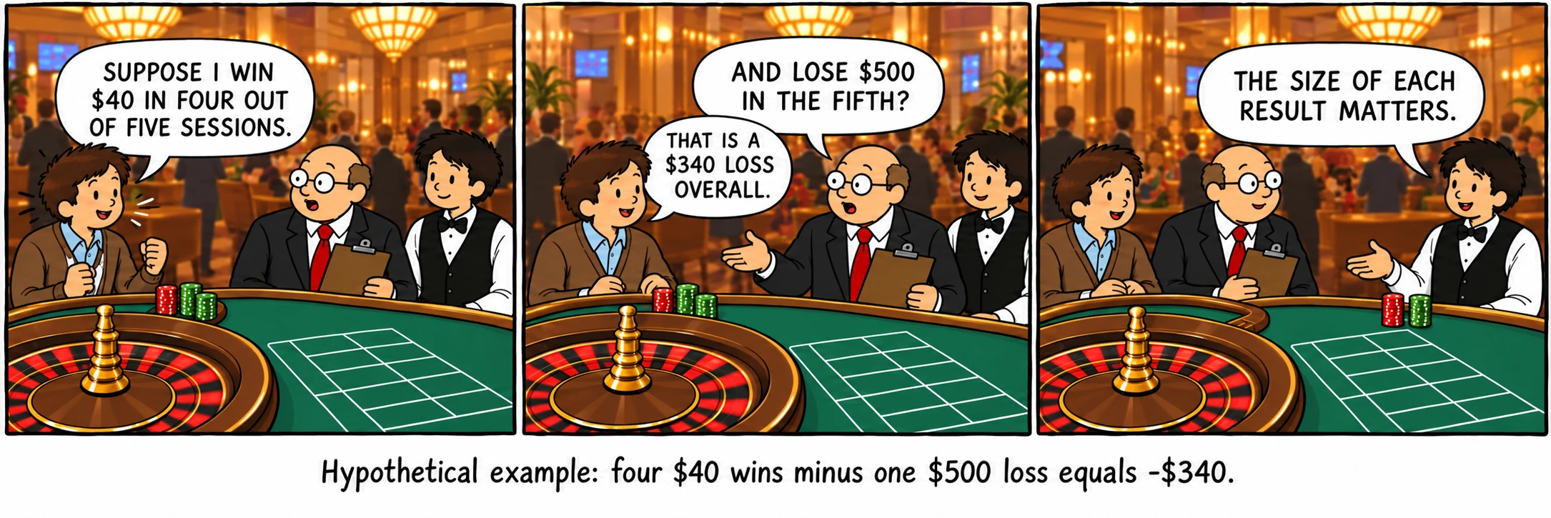
Hypothetical example: four $40 wins minus one $500 loss equals −$340.
ꯍꯧꯔꯛꯐꯃꯁꯤꯡ
- Thorp, E. O. “Optimal gambling systems for favorable games.”
- Thorp, E. O. The Mathematics of Gambling.
- Doob, J. L. “Note on probability.”
- Halmos, P. R. “Invariants of certain stochastic transformations: the mathematical theory of gambling systems.”
- Ethier, S. N. The Doctrine of Chances: Probabilistic Aspects of Gambling.
- Bollman, M. Mathematics of the Big Four Casino Table Games: Blackjack, Baccarat, Craps, & Roulette.
- Bollman, M. Basic Gambling Mathematics: The Numbers Behind the Neon, 2nd ed.