ꯔꯨꯂꯦꯠꯀꯤ ꯁ꯭ꯇꯦꯟꯗꯔꯗ ꯗꯤꯚꯤꯌꯦꯁꯟ
ꯔꯨꯂꯦꯠꯀꯤ ꯁ꯭ꯇꯦꯟꯗꯔꯗ ꯗꯤꯚꯤꯌꯦꯁꯟ, ꯚꯦꯌꯔꯤꯌꯦꯟꯁꯃꯦꯊꯃꯦꯇꯤꯛꯁꯚꯦꯌꯔꯤꯌꯦꯟꯁꯃꯍꯩꯁꯤꯡ ꯐꯪꯒꯗꯕ ꯃꯃꯂꯒꯤ ꯑꯀꯣꯌꯕꯗ ꯀꯌꯥ ꯁꯟꯗꯣꯛꯅ ꯂꯩꯕꯒꯦ ꯍꯥꯌꯕꯒꯤ ꯆꯥꯡ꯫ ꯁ꯭ꯇ꯭ꯔꯦꯠ-ꯑꯞꯇ ꯋꯥꯡꯏ, ꯆꯞ ꯃꯥꯟꯅꯕ ꯕꯦꯠꯁꯤꯡꯗ ꯅꯦꯝꯏ꯫ꯃꯄꯨꯡ ꯄꯥꯕꯤꯌꯨ →ꯀꯤ ꯁ꯭ꯀ꯭ꯋꯦꯌꯔ ꯔꯨꯠ, ꯑꯁꯤ ꯃꯍꯩ ꯑꯃꯥ ꯑꯃꯁꯨꯡ ꯃꯗꯨꯗꯒꯤ ꯐꯪꯒꯗꯕꯒꯤ ꯃꯔꯛꯇ ꯃꯍꯧꯁꯥꯅ ꯂꯩꯕ ꯂꯥꯞꯄꯅꯤ꯫
Per $1 staked, σ is 5.84 for a straight upꯕꯦꯠꯁ꯭ꯇ꯭ꯔꯦꯠ-ꯑꯞꯃꯁꯤꯡ ꯑꯃꯈꯛꯇ, 35:1 ꯄꯦꯑꯥꯎꯠ꯫ꯃꯄꯨꯡ ꯄꯥꯕꯤꯌꯨ → and 1.00 for red. For independent spinsꯃꯦꯊꯃꯦꯇꯤꯛꯁꯃꯔꯤ ꯂꯩꯅꯗꯕ ꯁ꯭ꯄꯤꯟꯁꯤꯡꯍꯥꯟꯅꯒꯤ ꯃꯍꯩ ꯀꯔꯤꯒꯨꯝꯕ ꯑꯣꯏꯔꯕꯁꯨ ꯁ꯭ꯄꯤꯟ ꯈꯨꯗꯤꯡꯃꯛꯀꯤ ꯊꯣꯛꯄꯒꯤ ꯈꯨꯗꯣꯡꯆꯥꯕ ꯃꯥꯟꯅꯩ꯫ ꯋꯦꯕꯁꯥꯏꯠ ꯑꯁꯤꯒꯤ ꯊꯤꯕ ꯈꯨꯗꯤꯡꯃꯛꯀꯤ ꯌꯨꯝꯐꯝꯅꯤ꯫ꯃꯄꯨꯡ ꯄꯥꯕꯤꯌꯨ → with the same bet and stake, multiply by the stake and the square root of the number of spins.
ꯂꯥꯏꯕ ꯅꯤꯌꯝ
When a normal approximation is suitable, about 68% of results lie within one standard deviationꯃꯦꯊꯃꯦꯇꯤꯛꯁꯁ꯭ꯇꯦꯟꯗꯔꯗ ꯗꯤꯚꯤꯌꯦꯁꯟꯚꯦꯌꯔꯤꯌꯦꯟꯁꯀꯤ ꯁ꯭ꯀ꯭ꯋꯦꯌꯔ ꯔꯨꯠ; ꯃꯍꯩ ꯑꯃꯅ ꯐꯪꯒꯗꯕ ꯃꯃꯜꯗꯒꯤ ꯌꯥꯝꯅ ꯂꯥꯞꯄ ꯃꯑꯣꯡ꯫ꯃꯄꯨꯡ ꯄꯥꯕꯤꯌꯨ → of the mean and 95% within two. These are approximations, not universal rules. For 100 independent $10 bets on redꯕꯦꯠꯑꯉꯥꯡꯕꯑꯉꯥꯡꯕ ꯃꯁꯤꯡ 18 ꯗ ꯊꯝꯕ ꯆꯞ ꯃꯥꯟꯅꯕ ꯕꯦꯠ꯫ ꯐ꯭ꯔꯦꯟꯆ: ꯔꯨꯖ꯫ꯃꯄꯨꯡ ꯄꯥꯕꯤꯌꯨ →, the expected result is about −$27 and the standard deviation is $100. The exact binomial probabilities below account for the fact that final results come in $20 steps. An unusual session alone does not establish an advantage.
ꯀꯔꯤꯒꯤ √N
Expected lossꯃꯦꯊꯃꯦꯇꯤꯛꯁꯃꯥꯡꯒꯗꯕ ꯁꯦꯜꯐꯪꯒꯗꯕ ꯃꯃꯂꯕꯨ ꯕꯦꯠ ꯊꯝꯂꯕ ꯁꯦꯜ ꯄꯨꯝꯅꯃꯛꯅ ꯃꯅꯥꯡꯕ; ꯁꯦꯁꯟ ꯅꯠꯔꯒ ꯃꯇꯝ ꯑꯃꯒꯤ ꯃꯅꯨꯡꯗ ꯃꯥꯡꯕ ꯑꯦꯚꯔꯦꯖ ꯁꯦꯜ꯫ꯃꯄꯨꯡ ꯄꯥꯕꯤꯌꯨ → grows in proportion to N; spread grows in proportion to √N. For short sessions, random variation can be large compared with the expected loss. As N grows, expected loss becomes larger relative to that spread. The crossover, where expected loss equals one standard deviation, is at N = (σ/edge)². Using unrounded single-zeroꯆꯛꯔꯖꯤꯔꯣꯆꯞ ꯃꯥꯟꯅꯕ, ꯗꯖꯟ ꯅꯠꯔꯒ ꯀꯂꯝ ꯕꯦꯠ ꯑꯃꯠꯇꯅ ꯀꯨꯞꯇꯕ ꯑꯁꯪꯕ ꯄꯣꯀꯦꯠ ꯑꯃꯈꯛꯇ; ꯍꯥꯎꯁ ꯑꯦꯖꯀꯤ ꯍꯧꯔꯀꯐꯝꯅꯤ꯫ ꯑꯇꯣꯞꯄ ꯃꯃꯤꯡ: ꯁꯤꯡꯒꯜ ꯖꯤꯔꯣ, 0꯫ꯃꯄꯨꯡ ꯄꯥꯕꯤꯌꯨ → values gives 1,368 spins for even-money betsꯕꯦꯠꯆꯞ ꯃꯥꯟꯅꯕ ꯕꯦꯠꯑꯉꯥꯡꯕ/ꯑꯃꯨꯕ, ꯕꯤꯖꯣꯔ/ꯖꯣꯔ, ꯑꯋꯥꯡꯕ/ꯑꯅꯦꯝꯕ꯫ ꯃꯁꯤꯡ 18, 1:1 ꯄꯦꯑꯥꯎꯠ꯫ꯃꯄꯨꯡ ꯄꯥꯕꯤꯌꯨ → and 46,656 for straight-up bets. This is a comparison of scales, not a point at which outcomes become certain.
ꯁꯤꯖꯤꯟꯅꯕ
To judge whether a session was unusual, compute (result − EV)/σ. A $10 red bettor who finishes 100 spins at +$160 has won 58 spins and lost 42. That result is about (160 + 27)/100 = 1.87 standard deviations above the mean. The exact probabilityꯃꯦꯊꯃꯦꯇꯤꯛꯁꯊꯣꯛꯄꯒꯤ ꯈꯨꯗꯣꯡꯆꯥꯕꯃꯍꯩ ꯑꯃꯥ ꯊꯣꯛꯄꯒꯤ ꯈꯨꯗꯣꯡꯆꯥꯕ, 0 ꯗꯒꯤ 1 ꯐꯥꯑꯣꯕ ꯅꯠꯔꯒ 0% ꯗꯒꯤ 100% ꯐꯥꯑꯣꯕ꯫ ꯃꯁꯤꯡ ꯑꯃꯥ: 1/37 = 2.70%꯫ꯃꯄꯨꯡ ꯄꯥꯕꯤꯌꯨ → of finishing at +$160 or better is about 3.82%. The z-score describes distance from the mean; use the actual outcome distribution to calculate a tail probability.
ꯆꯥꯡ ꯑꯃꯒꯤ ꯁ꯭ꯇꯦꯟꯗꯔꯗ ꯑꯦꯔꯔ
ꯃꯁꯤꯡ ꯊꯤꯖꯤꯟꯕ ꯑꯁꯤꯃꯛꯅ ꯗꯦꯇꯥꯗ ꯑꯦꯖ ꯎꯅꯕ ꯁ꯭ꯄꯤꯟ ꯀꯌꯥ ꯃꯊꯧ ꯇꯥꯕꯒꯦ ꯍꯥꯌꯕꯁꯨ ꯇꯥꯀꯏ꯫ ꯎꯈꯤꯕ ꯃꯥꯏꯄꯥꯛꯄꯒꯤ ꯆꯥꯡ ꯑꯃꯒꯤ ꯁ꯭ꯇꯦꯟꯗꯔꯗ ꯑꯦꯔꯔ √(p(1 − p)/N) ꯅꯤ꯫ N = 1,000 ꯂꯩꯕ ꯑꯉꯥꯡꯕꯗ: √(0.4865 × 0.5135 / 1000) ≈ 1.6%꯫ ꯆꯨꯝꯃꯤꯟꯅꯕ ꯀꯣꯏꯟ ꯑꯃꯁꯨꯡ ꯑꯉꯥꯡꯕꯒꯤ ꯃꯔꯛꯇ ꯂꯩꯕ ꯈꯦꯠꯅꯕ 1.35% ꯅꯤ, ꯃꯔꯝ ꯑꯗꯨꯅ ꯁ꯭ꯄꯤꯟ 1,000 ꯒꯤ ꯃꯇꯨꯡꯗꯁꯨ ꯃꯈꯣꯌ ꯊꯥꯖꯕꯥ ꯌꯥꯅꯅ ꯈꯦꯟꯗꯣꯛꯄ ꯉꯝꯗ꯭ꯔꯤ꯫ 10,000 ꯒꯤ ꯃꯇꯨꯡꯗ ꯁ꯭ꯇꯦꯟꯗꯔꯗ ꯑꯦꯔꯔ 0.5% ꯑꯣꯏ ꯑꯃꯁꯨꯡ ꯈꯦꯟꯗꯣꯛꯄ ꯉꯝꯃꯤ꯫ ꯆꯛꯔꯒꯤ ꯕꯥꯏꯌꯥꯁ ꯊꯤꯗꯣꯛꯅꯕ ꯁ꯭ꯄꯤꯟ ꯌꯥꯝꯅꯥ ꯀꯌꯥ ꯃꯊꯧ ꯇꯥꯕꯒꯤ ꯃꯔꯃꯁꯨ ꯃꯁꯤꯅꯤ꯫
ꯌꯦꯟꯊꯕꯒꯤ ꯃꯇꯥꯡꯗ ꯆꯦꯀꯁꯤꯅꯕ
Straight-up results are far from normally distributed in a short session: most sessions are a steady −$10 per spin with occasional +$350 jumps. The standard deviation remains valid, but the normal 68%/95% rule can be misleading. For even-money bets, the normal approximation becomes more useful as the number of spins grows; an exact binomial calculation avoids approximation error.
ꯐꯣꯔꯃꯨꯂꯥ
ꯋꯥꯍꯪꯁꯤꯡ
ꯃꯁꯤ ꯅꯍꯥꯛꯅ ꯁꯦꯁꯟ 40 ꯃꯔꯛ ꯁꯥꯅꯈꯤ, ꯅꯠꯔꯒ ꯃꯔꯤꯆꯥꯗꯒꯤ ꯂꯥꯛ ꯐꯕ ꯑꯃꯗ ꯂꯩꯈꯤ ꯍꯥꯌꯕꯒꯤ ꯁꯥꯛꯁꯤꯅꯤ꯫ ꯑꯃꯨꯛ ꯍꯟꯅꯥ ꯇꯧꯕꯤꯌꯨ꯫
For independent spins with a fixed bet and stake, the standard error of the average is σ/√N. At 10,000 spins it is about 1% of the stake for red, but about 5.84% for a straight-up bet. The spread shrinks with N; the observed average need not move steadily toward its expectation.
ꯃꯦꯊꯃꯦꯇꯤꯛꯁꯀꯥ ꯁꯥꯟꯅꯕ
ꯃꯁꯤꯁꯤꯡ ꯑꯍꯥꯅꯕꯗ ꯅꯍꯥꯛ ꯃꯁꯥꯃꯛꯅ ꯍꯣꯠꯅꯕꯤꯌꯨ꯫ ꯄꯥꯎꯈꯨꯝ ꯈꯨꯗꯤꯡꯃꯛ ꯊꯨꯡꯗꯨꯅ ꯊꯝꯂꯤ; ꯁꯦꯝ ꯁꯥꯔꯕ ꯃꯇꯃꯗ ꯍꯥꯡꯗꯣꯛꯄꯤꯌꯨ꯫
ꯌꯨꯔꯣꯄꯤꯌꯟ ꯆꯛꯔ ꯑꯃꯒꯤ ꯁ꯭ꯄꯤꯟ 100 ꯗ, ꯑꯉꯥꯡꯕꯕꯦꯠꯑꯉꯥꯡꯕꯑꯉꯥꯡꯕ ꯃꯁꯤꯡ 18 ꯗ ꯊꯝꯕ ꯆꯞ ꯃꯥꯟꯅꯕ ꯕꯦꯠ꯫ ꯐ꯭ꯔꯦꯟꯆ: ꯔꯨꯖ꯫ꯃꯄꯨꯡ ꯄꯥꯕꯤꯌꯨ → ꯗ ꯌꯨꯅꯤꯠꯁꯦꯜꯌꯨꯅꯤꯠꯁꯤꯁ꯭ꯇꯦꯝ ꯅꯠꯔꯒ ꯁꯥꯟꯅꯔꯤꯕ ꯑꯃꯅ ꯁꯤꯖꯤꯟꯅꯕ ꯃꯔꯨꯑꯣꯏꯕ ꯊꯝꯂꯕ ꯁꯦꯜ꯫ ꯄ꯭ꯔꯣꯒ꯭ꯔꯦꯁꯅꯁꯤꯡ ꯌꯨꯅꯤꯠꯇ ꯁꯟꯗꯣꯛꯂꯤ, ꯃꯔꯝ ꯑꯗꯨꯅ ꯃꯈꯣꯌ ꯀꯔꯤꯒꯨꯝꯕ ꯇꯦꯕꯜꯗ ꯆꯠꯂꯤ꯫ꯃꯄꯨꯡ ꯄꯥꯕꯤꯌꯨ → ꯑꯃꯥ ꯃꯥꯏꯄꯥꯛꯄ 51 ꯅꯠꯔꯒꯥ ꯍꯦꯟꯅ ꯐꯪꯂꯕꯗꯤ ꯀꯥꯟꯅꯕꯗ ꯂꯩ, ꯑꯃꯁꯨꯡ ꯁ꯭ꯇ꯭ꯔꯦꯠ-ꯑꯞꯕꯦꯠꯁ꯭ꯇ꯭ꯔꯦꯠ-ꯑꯞꯃꯁꯤꯡ ꯑꯃꯈꯛꯇ, 35:1 ꯄꯦꯑꯥꯎꯠ꯫ꯃꯄꯨꯡ ꯄꯥꯕꯤꯌꯨ → ꯗ ꯌꯨꯅꯤꯠ ꯑꯃꯥ ꯃꯁꯤꯒꯤ ꯃꯁꯤꯡ ꯑꯃꯨꯛ 3 ꯅꯠꯔꯒꯥ ꯍꯦꯟꯅ ꯊꯣꯛꯂꯕꯗꯤ ꯀꯥꯟꯅꯕꯗ ꯂꯩ꯫ ꯕꯦꯜ ꯀꯔꯚ ꯁꯤꯖꯤꯟꯅꯗꯨꯅ ꯈꯨꯗꯣꯡꯆꯥꯕ ꯑꯅꯤꯃꯛ ꯈꯟꯊꯕꯤꯌꯨ, ꯃꯗꯨꯒꯤ ꯃꯇꯨꯡꯗ ꯃꯈꯣꯌꯕꯨ ꯑꯆꯨꯝꯕ ꯄꯥꯎꯈꯨꯃꯁꯤꯡꯒꯥ ꯆꯥꯡꯗꯝꯕꯤꯌꯨ꯫
ꯄꯥꯎꯈꯨꯝ ꯎꯠꯄ
ꯄꯥꯎꯈꯨꯝ ꯑꯉꯥꯡꯕ: ꯕꯦꯜ ꯀꯔꯚꯅ 35.6% ꯄꯤ ꯑꯃꯁꯨꯡ ꯑꯆꯨꯝꯕ ꯄꯥꯎꯈꯨꯝ 35.5%꯫ ꯁ꯭ꯇ꯭ꯔꯦꯠ-ꯑꯞ: ꯕꯦꯜ ꯀꯔꯚꯅ 55.0% ꯄꯤ ꯑꯃꯁꯨꯡ ꯑꯆꯨꯝꯕ ꯄꯥꯎꯈꯨꯝ 50.9%꯫ ꯊꯨꯅ ꯍꯤꯁꯥꯕ ꯇꯧꯕ ꯑꯁꯤ ꯑꯉꯥꯡꯕꯒꯤꯗꯃꯛ ꯆꯨꯝꯃꯤ ꯑꯃꯁꯨꯡ ꯃꯁꯤꯡ ꯑꯃꯈꯛꯀꯤꯗꯃꯛ ꯆꯨꯃꯗꯦ꯫
ꯑꯉꯥꯡꯕ: ꯃꯥꯏꯄꯥꯛꯄꯒꯤ ꯑꯦꯚꯔꯦꯖ 100 × 18/37 = 48.6, ꯁ꯭ꯞꯔꯦꯗ √(100 × 18/37 × 19/37) = 5.0꯫ ꯀꯥꯟꯅꯕꯗ ꯂꯩꯕ ꯍꯥꯌꯕꯁꯤ 51 ꯅꯠꯔꯒꯥ ꯍꯦꯟꯅꯅꯤ; ꯃꯔꯛꯀꯤ ꯃꯐꯝ, 50.5, ꯑꯁꯤ ꯑꯦꯚꯔꯦꯖꯗꯒꯤ ꯁ꯭ꯞꯔꯦꯗ 0.37 ꯃꯊꯛꯇ ꯂꯩ, ꯑꯃꯁꯨꯡ ꯕꯦꯜ ꯀꯔꯚꯅ ꯃꯁꯤꯒꯤ ꯃꯊꯛꯇ 35.6% ꯊꯝꯏ꯫ ꯃꯥꯏꯄꯥꯛꯄ 51, 52 … 100 ꯒꯤ ꯑꯆꯨꯝꯕ ꯈꯨꯗꯣꯡꯆꯥꯕꯁꯤꯡ ꯄꯨꯟꯁꯤꯜꯂꯕꯗ 35.5% ꯄꯤ꯫
ꯁ꯭ꯇ꯭ꯔꯦꯠ-ꯑꯞ: ꯊꯣꯛꯄꯒꯤ ꯑꯦꯚꯔꯦꯖ 100/37 = 2.70, ꯁ꯭ꯞꯔꯦꯗ √(100 × 1/37 × 36/37) = 1.62꯫ ꯑꯍꯨꯝ ꯅꯠꯔꯒꯥ ꯍꯦꯟꯅ ꯊꯣꯛꯄ ꯍꯥꯌꯕꯁꯤ 2.5 ꯒꯤ ꯃꯊꯛꯇꯅꯤ, ꯑꯦꯚꯔꯦꯖꯗꯒꯤ ꯁ꯭ꯞꯔꯦꯗ 0.12 ꯃꯈꯥꯗ: ꯕꯦꯜ ꯀꯔꯚꯗ 55.0%꯫ ꯑꯆꯨꯝꯕꯗ, ꯃꯁꯤ 1 ꯗꯒꯤ ꯊꯣꯛꯄ 0, 1 ꯑꯃꯁꯨꯡ 2 ꯒꯤ ꯈꯨꯗꯣꯡꯆꯥꯕꯁꯤꯡ ꯂꯧꯊꯣꯀꯄꯅꯤ, 6.5% + 17.9% + 24.7%, ꯃꯁꯤꯅ 50.9% ꯊꯃꯖꯤꯜꯂꯤ꯫
ꯕꯦꯜ ꯀꯔꯚꯗ ꯑꯦꯚꯔꯦꯖꯀꯤ ꯃꯥꯏꯀꯩ ꯑꯅꯤꯃꯛꯇ ꯃꯍꯩ ꯌꯥꯝꯅꯥ ꯃꯊꯧ ꯇꯥꯏ꯫ ꯁ꯭ꯄꯤꯟ 100 ꯒꯤ ꯃꯇꯨꯡꯗ ꯑꯉꯥꯡꯕꯗ ꯃꯈꯣꯌ ꯂꯩ; ꯑꯦꯚꯔꯦꯖꯗ ꯑꯃꯨꯛ ꯑꯍꯨꯃꯗꯒꯤ ꯍꯟꯊꯅ ꯊꯣꯛꯄ ꯃꯁꯤꯡ ꯑꯃꯗ ꯂꯩꯇꯦ꯫ ꯀꯔꯚ ꯑꯁꯤꯅ “ꯊꯣꯛꯄ ꯑꯃꯠꯇ ꯂꯩꯇꯕ” ꯑꯗꯨꯗꯁꯨ 8.7% ꯄꯤ, ꯑꯆꯨꯝꯕ ꯈꯨꯗꯣꯡꯆꯥꯕ 6.5% ꯑꯣꯏꯔꯤꯉꯩꯗ꯫ Taylor (2021) ꯅ ꯕꯥꯏꯅꯣꯃꯤꯌꯦꯜ ꯑꯃꯁꯨꯡ ꯕꯦꯜ ꯀꯔꯚ ꯑꯁꯤ ꯃꯑꯣꯡ ꯑꯗꯨꯃꯛꯇ ꯃꯅꯥꯛ ꯃꯅꯥꯛꯇ ꯊꯝꯃꯤ꯫
ꯅꯣꯛꯅꯕꯒꯤ ꯀꯃꯤꯛ
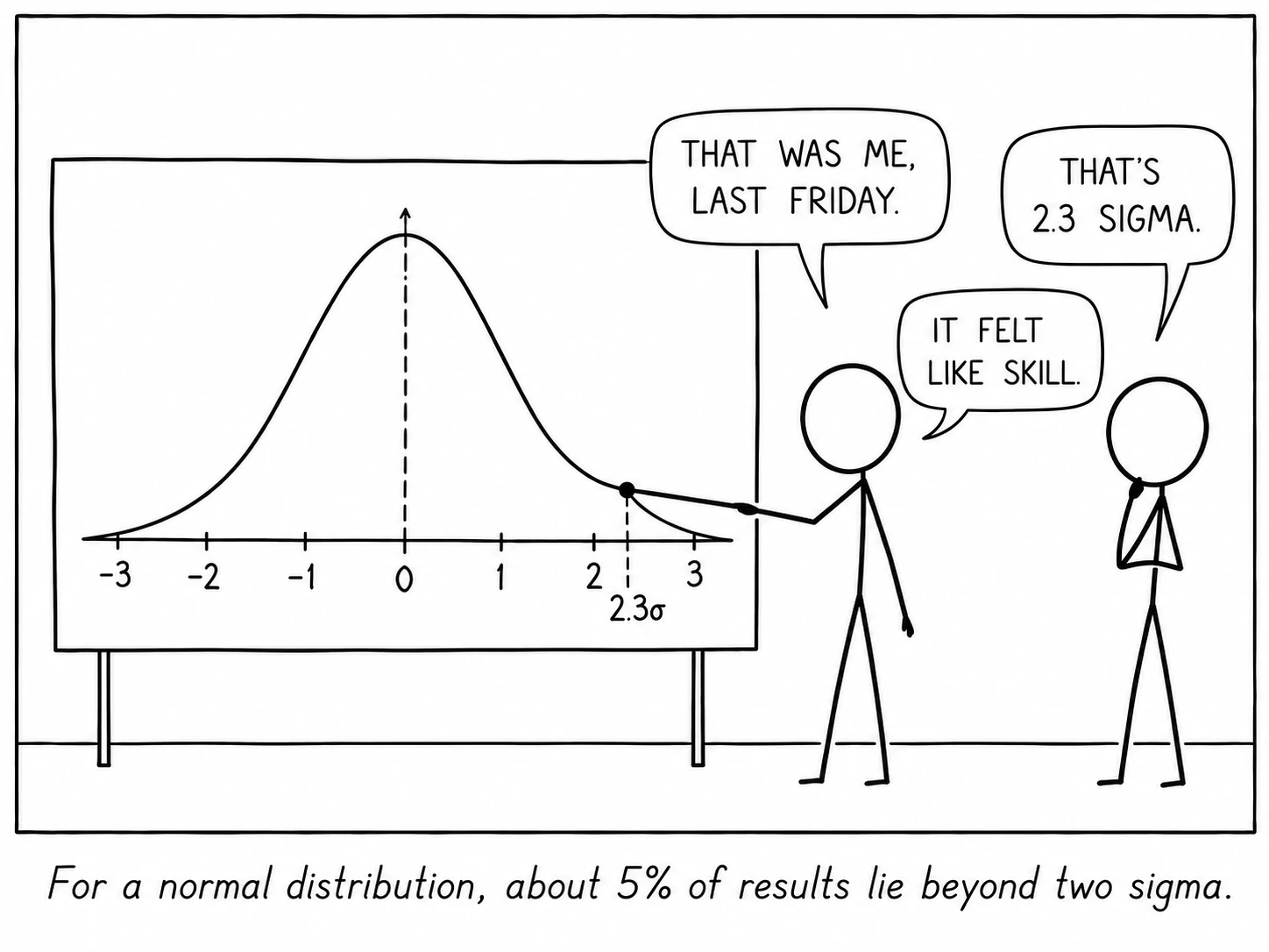
Under a normal approximation, about 5% of results lie more than two standard deviations from the mean.
ꯍꯧꯔꯛꯐꯃꯁꯤꯡ
- Feller, W. An Introduction to Probability Theory and Its Applications, Vol. 1.
- Ethier, S. N. The Doctrine of Chances: Probabilistic Aspects of Gambling.
- Taylor, D. G. Games, Gambling, and Probability: An Introduction to Mathematics, 2nd ed.