ꯃꯥꯡꯒꯗꯕ ꯁꯦꯜ
House edgeꯃꯦꯊꯃꯦꯇꯤꯛꯁꯍꯥꯎꯁ ꯑꯦꯖꯊꯝꯂꯕ ꯁꯦꯜ ꯈꯨꯗꯤꯡꯗꯒꯤ ꯀꯦꯁꯤꯅꯣꯅ ꯑꯦꯚꯔꯦꯖꯗ ꯊꯃꯖꯤꯜꯂꯤꯕ ꯁꯔꯨꯛ: ꯌꯨꯔꯣꯄꯤꯌꯟ ꯔꯨꯂꯦꯠꯇ 2.70%꯫ꯃꯄꯨꯡ ꯄꯥꯕꯤꯌꯨ → times the amount wagered: how to calculate expected loss.

ꯃꯥꯡꯒꯗꯕ ꯁꯦꯜ = ꯊꯝꯂꯕ ꯁꯦꯜ ꯄꯨꯝꯅꯃꯛ × 1/37꯫ $10 ꯊꯝꯗꯨꯅ ꯁ꯭ꯄꯤꯟ 100: $1,000 ꯊꯝꯂꯦ, ꯃꯥꯡꯒꯗꯕ ꯁꯦꯜ $27꯫ ꯄ꯭ꯔꯣꯒ꯭ꯔꯦꯁꯅꯁꯤꯡꯅ ꯍꯦꯟꯅꯥ ꯊꯝꯃꯤ, ꯃꯔꯝ ꯑꯗꯨꯅ ꯃꯈꯣꯌꯅ ꯍꯦꯟꯅꯥ ꯃꯥꯡꯏ꯫
ꯇꯔꯅꯑꯣꯚꯔꯅꯤ, ꯕꯦꯡꯀꯔꯣꯜ ꯅꯠꯇꯦ
Expected lossꯃꯦꯊꯃꯦꯇꯤꯛꯁꯃꯥꯡꯒꯗꯕ ꯁꯦꯜꯐꯪꯒꯗꯕ ꯃꯃꯂꯕꯨ ꯕꯦꯠ ꯊꯝꯂꯕ ꯁꯦꯜ ꯄꯨꯝꯅꯃꯛꯅ ꯃꯅꯥꯡꯕ; ꯁꯦꯁꯟ ꯅꯠꯔꯒ ꯃꯇꯝ ꯑꯃꯒꯤ ꯃꯅꯨꯡꯗ ꯃꯥꯡꯕ ꯑꯦꯚꯔꯦꯖ ꯁꯦꯜ꯫ꯃꯄꯨꯡ ꯄꯥꯕꯤꯌꯨ → depends on how much passes across the table, not on how much you brought. Completing $2,000 of standard single-zeroꯆꯛꯔꯖꯤꯔꯣꯆꯞ ꯃꯥꯟꯅꯕ, ꯗꯖꯟ ꯅꯠꯔꯒ ꯀꯂꯝ ꯕꯦꯠ ꯑꯃꯠꯇꯅ ꯀꯨꯞꯇꯕ ꯑꯁꯪꯕ ꯄꯣꯀꯦꯠ ꯑꯃꯈꯛꯇ; ꯍꯥꯎꯁ ꯑꯦꯖꯀꯤ ꯍꯧꯔꯀꯐꯝꯅꯤ꯫ ꯑꯇꯣꯞꯄ ꯃꯃꯤꯡ: ꯁꯤꯡꯒꯜ ꯖꯤꯔꯣ, 0꯫ꯃꯄꯨꯡ ꯄꯥꯕꯤꯌꯨ → bets gives an expected loss of $54.05. A $100 starting bankrollꯁꯦꯜꯕꯦꯡꯀꯔꯣꯜꯁꯥꯟꯅꯅꯕ ꯇꯣꯉꯥꯟꯅ ꯊꯝꯂꯕ ꯁꯦꯜ ꯄꯨꯝꯅꯃꯛ꯫ ꯕꯦꯡꯀꯔꯣꯜ ꯃꯦꯅꯦꯖꯃꯦꯟꯠ ꯍꯥꯌꯕꯁꯤ ꯃꯗꯨꯒꯤ ꯀꯌꯥ ꯕꯦꯠ ꯈꯨꯗꯤꯡꯗ ꯑꯃꯁꯨꯡ ꯁꯦꯁꯟ ꯈꯨꯗꯤꯡꯗ ꯈꯨꯗꯣꯡꯊꯤꯕꯗ ꯊꯃꯒꯗꯒꯦ ꯍꯥꯌꯕ ꯋꯥꯔꯦꯞ ꯂꯧꯕꯅꯤ꯫ꯃꯄꯨꯡ ꯄꯥꯕꯤꯌꯨ → might or might not last long enough to complete that turnoverꯁꯦꯜꯇꯔꯅꯑꯣꯚꯔꯁꯦꯁꯟ ꯅꯠꯔꯒ ꯃꯇꯝ ꯑꯃꯒꯤ ꯃꯅꯨꯡꯗ ꯕꯦꯠ ꯊꯝꯂꯕ ꯁꯦꯜ ꯄꯨꯝꯅꯃꯛ, ꯑꯃꯨꯛ ꯍꯟꯅꯥ ꯊꯝꯂꯕ ꯃꯥꯏꯄꯥꯛꯇꯨꯅ ꯐꯪꯂꯕ ꯁꯦꯜꯁꯨ ꯌꯥꯎꯅ꯫ ꯑꯇꯣꯞꯄ ꯃꯃꯤꯡ: ꯍꯦꯟꯗꯜ, ꯑꯦꯛꯁꯟ꯫ꯃꯄꯨꯡ ꯄꯥꯕꯤꯌꯨ →. A single $10,000 bet on redꯕꯦꯠꯑꯉꯥꯡꯕꯑꯉꯥꯡꯕ ꯃꯁꯤꯡ 18 ꯗ ꯊꯝꯕ ꯆꯞ ꯃꯥꯟꯅꯕ ꯕꯦꯠ꯫ ꯐ꯭ꯔꯦꯟꯆ: ꯔꯨꯖ꯫ꯃꯄꯨꯡ ꯄꯥꯕꯤꯌꯨ → has an expected loss of $270.27. These are averages, not deductions or limits on the actual loss.
ꯐꯣꯔꯃꯨꯂꯥ
For a fixed schedule of standard single-zero bets, E[loss] = total stakes / 37. With stakes or stopping times that depend on earlier results, expected loss is expected turnover / 37, provided expected turnover is finite. The table shows fixed-stake examples, assuming all 100 spins are completed. Progressionꯊꯧꯔꯥꯡꯄ꯭ꯔꯣꯒ꯭ꯔꯦꯁꯟꯃꯃꯥꯡꯒꯤ ꯃꯍꯩꯁꯤꯡꯒꯤ ꯃꯈꯥꯗ ꯊꯝꯂꯕ ꯁꯦꯜ ꯍꯣꯡꯍꯟꯕ ꯅꯤꯌꯝ ꯀꯔꯤꯒꯨꯝꯕ꯫ ꯅꯦꯒꯦꯇꯤꯕ ꯄ꯭ꯔꯣꯒ꯭ꯔꯦꯁꯅꯁꯤꯡꯅ ꯃꯥꯏꯊꯤꯔꯕꯥ ꯃꯇꯨꯡꯗ ꯍꯦꯅꯒꯠꯍꯜꯂꯤ, ꯄꯣꯖꯤꯇꯤꯕꯁꯤꯡꯅ ꯃꯥꯏꯄꯥꯛꯂꯕꯥ ꯃꯇꯨꯡꯗ꯫ꯃꯄꯨꯡ ꯄꯥꯕꯤꯌꯨ → averages require a specified bankroll, limit, stopping rule and simulation or calculation.
ꯊꯨꯅꯕ
ꯂꯥꯏꯕ ꯇꯦꯕꯜꯁꯤꯡꯅ ꯄꯨꯡ ꯑꯃꯗ ꯁ꯭ꯄꯤꯟ 40–60 ꯆꯂꯥꯏ, ꯀꯦꯁꯤꯅꯣ ꯐ꯭ꯂꯣꯔꯁꯤꯡꯅ 30–50, ꯁ꯭ꯄꯤꯗ ꯇꯦꯕꯜꯁꯤꯡꯅ 90 ꯅꯠꯔꯒ ꯍꯦꯟꯅꯥ, RNG ꯇꯦꯕꯜꯁꯤꯡꯅ ꯅꯍꯥꯛꯅ ꯀ꯭ꯂꯤꯛ ꯇꯧꯕ ꯌꯥꯕꯃꯛ ꯊꯨꯅ꯫ ꯊꯝꯂꯕ ꯁꯦꯜ ꯃꯥꯟꯅꯔꯕꯗ ꯊꯨꯅꯕ ꯑꯁꯤ ꯄꯨꯡ ꯈꯨꯗꯤꯡꯒꯤ ꯃꯥꯡꯒꯗꯕ ꯁꯦꯜꯗ ꯈ꯭ꯕꯥꯏꯗꯒꯤ ꯆꯥꯎꯕ ꯁꯣꯀꯍꯟꯕꯅꯤ: ꯇꯞꯅ ꯆꯠꯂꯤꯕ ꯐ꯭ꯂꯣꯔ ꯇꯦꯕꯜ ꯑꯃꯗꯒꯤ ꯄꯨꯡ ꯑꯃꯗ ꯁ꯭ꯄꯤꯟ 200 ꯁꯥꯟꯅꯕ RNG ꯇꯦꯕꯜ ꯑꯃꯗ ꯆꯠꯄꯅ ꯑꯣꯗꯁ ꯀꯔꯤꯁꯨ ꯍꯣꯡꯗꯅ ꯅꯨꯃꯤꯗꯥꯡꯒꯤ ꯃꯃꯜ ꯃꯔꯤ ꯊꯥꯛ ꯍꯦꯅꯒꯠꯍꯜꯂꯤ꯫
ꯆꯍꯤ ꯑꯃꯗ
At 50 spins per hour, two hours per week and $10 per spin for 52 weeks, total turnover is $52,000. Expected loss is about $1,405 on standard single-zero bets, $703 on la partageꯅꯤꯌꯝꯂꯥ ꯄꯥꯔꯇꯥꯖꯐ꯭ꯔꯦꯟꯆ ꯅꯤꯌꯝ: ꯖꯤꯔꯣ ꯊꯣꯛꯂꯕꯗꯤ ꯆꯞ ꯃꯥꯟꯅꯕ ꯕꯦꯠꯀꯤ ꯊꯝꯂꯕ ꯁꯦꯜꯒꯤ ꯁꯔꯨꯛ ꯑꯍꯦꯟꯕ ꯍꯜꯂꯀꯏ꯫ ꯕꯦꯠ ꯑꯗꯨꯁꯤꯡꯒꯤ ꯍꯥꯎꯁ ꯑꯦꯖ 1.35% ꯐꯥꯑꯣꯕ ꯁꯔꯨꯛ ꯑꯅꯤꯗ ꯊꯥꯖꯤꯜꯂꯤ꯫ꯃꯄꯨꯡ ꯄꯥꯕꯤꯌꯨ → even-money betsꯕꯦꯠꯆꯞ ꯃꯥꯟꯅꯕ ꯕꯦꯠꯑꯉꯥꯡꯕ/ꯑꯃꯨꯕ, ꯕꯤꯖꯣꯔ/ꯖꯣꯔ, ꯑꯋꯥꯡꯕ/ꯑꯅꯦꯝꯕ꯫ ꯃꯁꯤꯡ 18, 1:1 ꯄꯦꯑꯥꯎꯠ꯫ꯃꯄꯨꯡ ꯄꯥꯕꯤꯌꯨ →, or $2,737 on standard double-zero bets other than the five-number bet. These figures assume every scheduled bet is made. Fewer bets, smaller stakes or a lower edge reduce expected loss; actual results remain uncertain.
ꯀꯔꯤꯒꯨꯝꯕ ꯕꯦꯡꯛ ꯑꯃꯗꯒꯤ ꯍꯦꯟꯅꯥ ꯃꯃꯜ ꯂꯩꯕ ꯁꯥꯟꯅꯕ ꯑꯃꯥ
The St. Petersburg game, posed by Nicolaus Bernoulli in 1713, tosses a coin until it lands heads and pays $2 if that takes one toss, $4 if two, $8 if three, doubling each time. Every possible length adds $1 to the expected valueꯃꯦꯊꯃꯦꯇꯤꯛꯁꯐꯪꯒꯗꯕ ꯃꯃꯜꯃꯇꯝ ꯁꯥꯡꯅ ꯌꯦꯡꯂꯕꯗ ꯕꯦꯠ ꯑꯃꯒꯤ ꯑꯦꯚꯔꯦꯖ ꯃꯍꯩ꯫ ꯃꯔꯨꯑꯣꯏꯕ ꯌꯨꯔꯣꯄꯤꯌꯟ ꯕꯦꯠ ꯈꯨꯗꯤꯡꯗ ꯊꯝꯂꯕ ꯁꯦꯜꯒꯤ −1/37꯫ꯃꯄꯨꯡ ꯄꯥꯕꯤꯌꯨ →, so on paper the game is worth an infinite amount. No bank can pay infinite prizes, and once the prizes are capped at what the bank holds, the value collapses: with a bank of $1 million the game is worth about $21, with $1 billion about $31. The comparison with Martingaleꯊꯧꯔꯥꯡꯃꯥꯔꯇꯤꯟꯒꯦꯜꯃꯥꯏꯊꯤꯕ ꯈꯨꯗꯤꯡꯒꯤ ꯃꯇꯨꯡꯗ ꯕꯦꯠ ꯑꯗꯨ ꯑꯅꯤ ꯊꯥꯛ ꯍꯦꯅꯒꯠꯍꯟꯕ ꯄ꯭ꯔꯣꯒ꯭ꯔꯦꯁꯟ꯫ ꯃꯁꯤꯅ ꯀꯔꯤ ꯇꯧꯕꯒꯦ ꯑꯃꯁꯨꯡ ꯀꯔꯤ ꯇꯧꯗꯕꯒꯦ ꯍꯥꯌꯕ ꯊꯧꯔꯥꯡꯒꯤ ꯁꯦꯛꯁꯅꯗ ꯌꯦꯡꯕꯤꯌꯨ꯫ꯃꯄꯨꯡ ꯄꯥꯕꯤꯌꯨ → is the importance of limits: a theoretical doubling sequence can require stakes beyond any finite bankroll or table limitꯇꯦꯕꯜꯇꯦꯕꯜꯒꯤ ꯉꯝꯈꯩꯌꯥꯍꯜꯂꯤꯕ ꯈ꯭ꯕꯥꯏꯗꯒꯤ ꯅꯦꯝꯕ ꯑꯃꯁꯨꯡ ꯈ꯭ꯕꯥꯏꯗꯒꯤ ꯋꯥꯡꯕ ꯕꯦꯠ꯫ ꯈ꯭ꯕꯥꯏꯗꯒꯤ ꯋꯥꯡꯕ ꯉꯝꯈꯩ ꯑꯗꯨꯅ ꯑꯅꯤ ꯊꯥꯛ ꯍꯦꯅꯒꯠꯍꯟꯕ ꯄ꯭ꯔꯣꯒ꯭ꯔꯦꯁꯅꯁꯤꯡ ꯊꯤꯡꯏ꯫ꯃꯄꯨꯡ ꯄꯥꯕꯤꯌꯨ →. That does not make the two games identical. A failed progression need not lose the entire bankroll, and a short session can finish ahead.
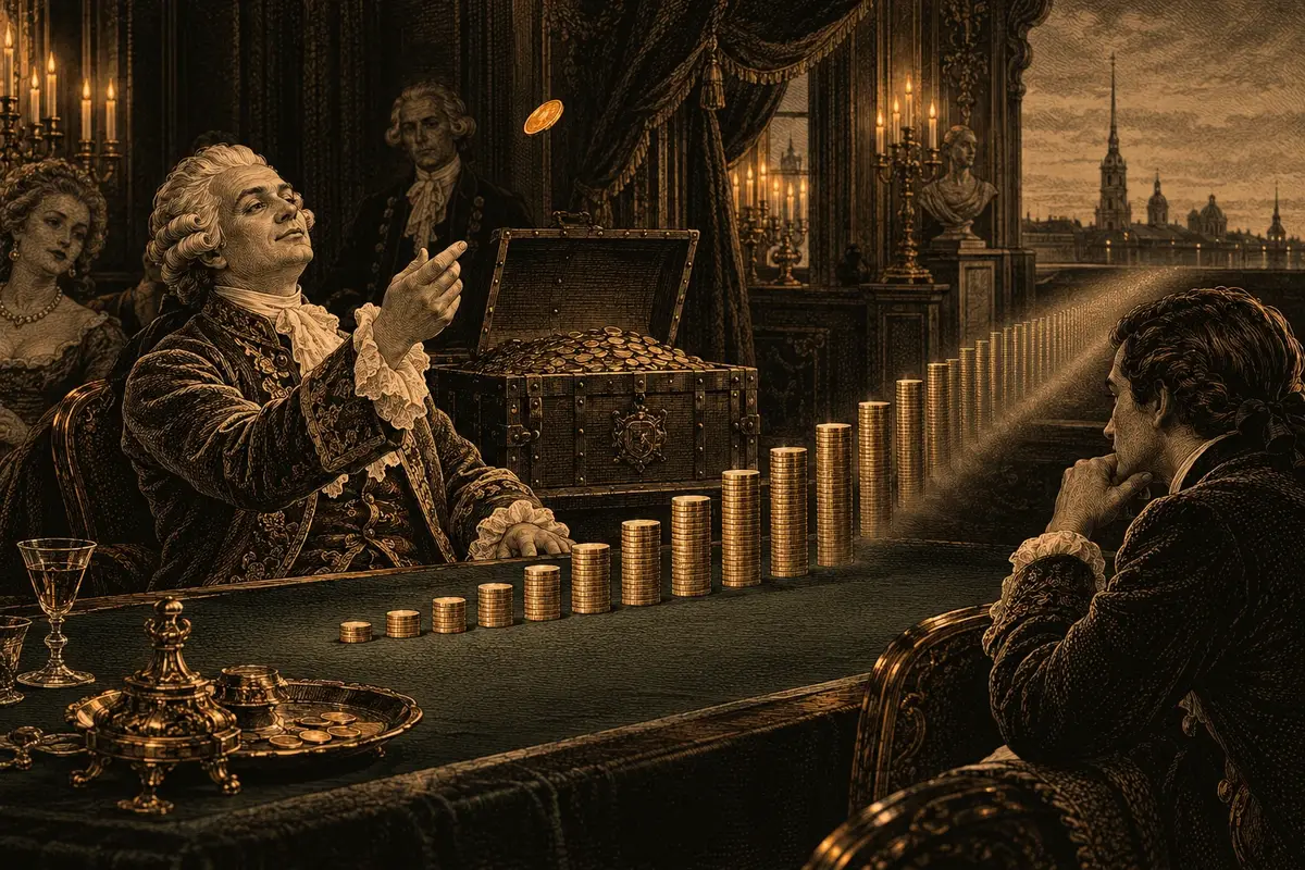
ꯃꯥꯡꯒꯗꯕ ꯁꯦꯜ ꯑꯁꯤ ꯃꯍꯩ ꯅꯠꯇꯦ
A single session can differ greatly from its expected loss. For 100 independent standard single-zero even-money bets at $10 each, the net result has a standard deviationꯃꯦꯊꯃꯦꯇꯤꯛꯁꯁ꯭ꯇꯦꯟꯗꯔꯗ ꯗꯤꯚꯤꯌꯦꯁꯟꯚꯦꯌꯔꯤꯌꯦꯟꯁꯀꯤ ꯁ꯭ꯀ꯭ꯋꯦꯌꯔ ꯔꯨꯠ; ꯃꯍꯩ ꯑꯃꯅ ꯐꯪꯒꯗꯕ ꯃꯃꯜꯗꯒꯤ ꯌꯥꯝꯅ ꯂꯥꯞꯄ ꯃꯑꯣꯡ꯫ꯃꯄꯨꯡ ꯄꯥꯕꯤꯌꯨ → of about $99.96 and an expected value of −$27.03. A winning session is possible. Expected loss describes the average across repeated sessions under those assumptions; it is neither a fee nor a limit on what one session can lose.
ꯐꯣꯔꯃꯨꯂꯥ
ꯋꯥꯍꯪꯁꯤꯡ
No fixed percentage is deducted from your buy-inꯇꯦꯕꯜꯕꯥꯏ-ꯏꯟꯇꯦꯕꯜꯗ ꯁꯦꯜ ꯄꯤꯗꯨꯅ ꯆꯤꯞꯁꯤꯡ ꯂꯧꯕ꯫ ꯁ꯭ꯄꯤꯟꯁꯤꯡꯒꯤ ꯃꯔꯛꯇ ꯇꯧꯏ, ꯁꯦꯜ ꯑꯗꯨ ꯗꯤꯂꯔꯒꯤ ꯈꯨꯠꯇ ꯄꯤꯗꯅ ꯂꯦꯑꯥꯎꯠꯇ ꯊꯝꯃꯤ꯫ꯃꯄꯨꯡ ꯄꯥꯕꯤꯌꯨ →. For standard bets on a fair single-zero wheel, expected loss is about 2.70% of the amount wagered. Actual results vary. Re-betting winnings adds to the amount wagered.
With the same rules and number of bets, a smaller fixed stake lowers expected loss. The probabilityꯃꯦꯊꯃꯦꯇꯤꯛꯁꯊꯣꯛꯄꯒꯤ ꯈꯨꯗꯣꯡꯆꯥꯕꯃꯍꯩ ꯑꯃꯥ ꯊꯣꯛꯄꯒꯤ ꯈꯨꯗꯣꯡꯆꯥꯕ, 0 ꯗꯒꯤ 1 ꯐꯥꯑꯣꯕ ꯅꯠꯔꯒ 0% ꯗꯒꯤ 100% ꯐꯥꯑꯣꯕ꯫ ꯃꯁꯤꯡ ꯑꯃꯥ: 1/37 = 2.70%꯫ꯃꯄꯨꯡ ꯄꯥꯕꯤꯌꯨ → of reaching a profit target is a different question and also depends on bankroll, stake and stopping rules.
ꯀꯦꯁꯤꯅꯣꯁꯤꯡꯅ ꯑꯦꯚꯔꯦꯖ ꯕꯦꯠ ꯑꯃꯁꯨꯡ ꯁꯥꯟꯅꯈꯤꯕ ꯃꯇꯃꯗꯒꯤ ꯅꯍꯥꯛꯀꯤ ꯃꯥꯡꯒꯗꯕ ꯁꯦꯜ ꯊꯤꯖꯤꯜꯂꯤ ꯑꯃꯁꯨꯡ ꯃꯗꯨꯒꯤ ꯁꯔꯨꯛ ꯈꯔꯥ ꯀꯣꯝꯞ (ꯃꯃꯜ ꯌꯥꯎꯗꯕ ꯈꯨꯗꯣꯜ) ꯑꯣꯏꯅ ꯍꯜꯂꯛꯏ꯫ ꯃꯈꯣꯌꯅ ꯃꯃꯂꯒꯤ ꯁꯔꯨꯛ ꯈꯔꯥ ꯍꯜꯂꯛꯂꯤꯕꯅꯤ, ꯅꯍꯥꯀꯄꯨ ꯑꯦꯖ ꯑꯃꯥ ꯄꯤꯔꯤꯕ ꯅꯠꯇꯦ꯫
ꯅꯣꯛꯅꯕꯒꯤ ꯀꯃꯤꯛ
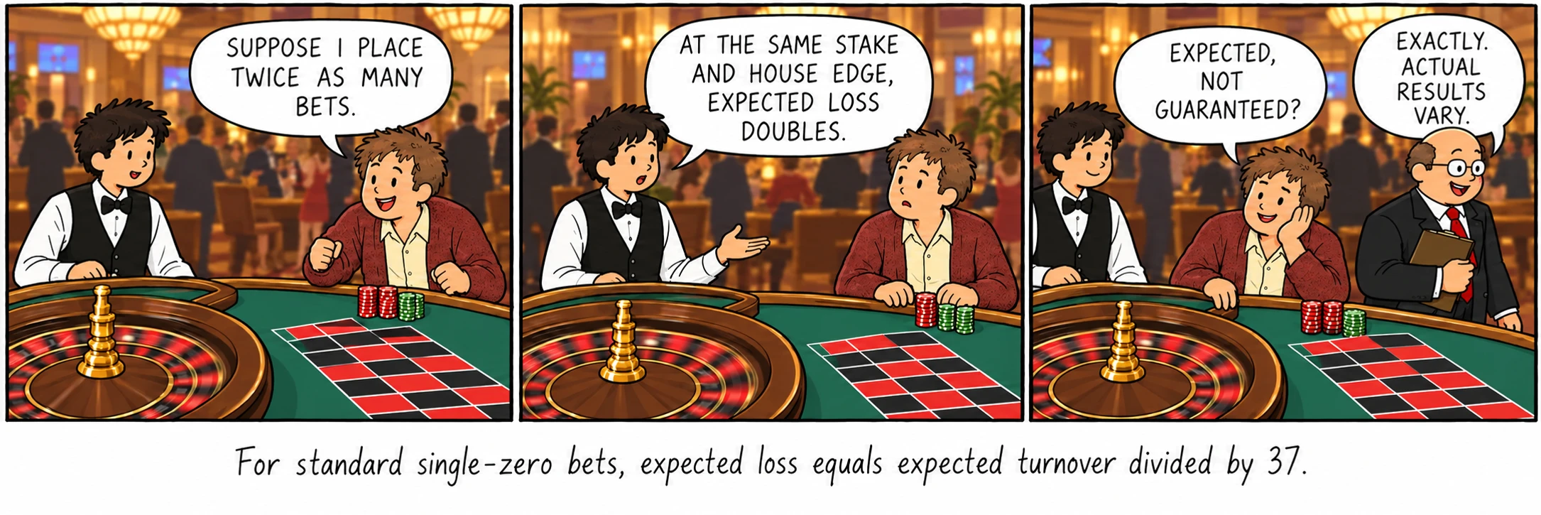
ꯇꯔꯅꯑꯣꯚꯔ × 1/37꯫ ꯄꯨꯡꯐꯝ ꯑꯁꯤ ꯐꯣꯔꯃꯨꯂꯥꯗ ꯌꯥꯎꯔꯤ꯫
ꯍꯧꯔꯛꯐꯃꯁꯤꯡ
- Ethier, S. N. The Doctrine of Chances: Probabilistic Aspects of Gambling.
- Epstein, R. A. The Theory of Gambling and Statistical Logic, 2nd ed.
- Taylor, D. G. Games, Gambling, and Probability: An Introduction to Mathematics, 2nd ed.