ꯔꯨꯂꯦꯠ ꯀꯝꯄꯤꯎꯇꯔꯁꯤꯡ
ꯀꯝꯄꯤꯎꯇꯔ ꯑꯃꯅ ꯕꯣꯜꯒꯤ ꯃꯇꯝ ꯀꯔꯝꯅ ꯊꯥꯖꯕꯒꯦ, ꯑꯍꯥꯅꯕꯁꯤꯡ ꯀꯅꯥꯅ ꯁꯦꯃꯈꯤꯕꯒꯦ, ꯑꯃꯁꯨꯡ ꯃꯁꯤ ꯀꯌꯥ ꯆꯨꯝꯒꯗꯒꯦ꯫
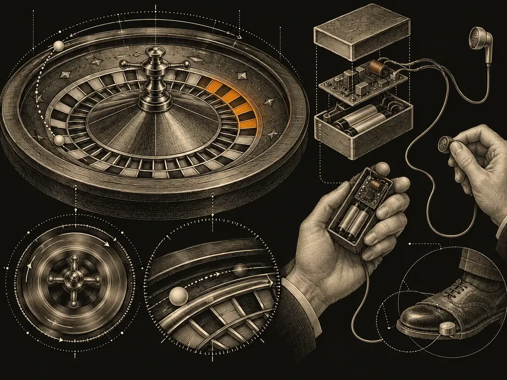
ꯔꯨꯂꯦꯠ ꯀꯝꯄꯤꯎꯇꯔ ꯑꯃꯅ ꯁ꯭ꯄꯤꯟ ꯑꯃꯒꯤ ꯑꯍꯥꯅꯕ ꯆꯦꯛꯀꯟꯗ ꯈꯔꯗ ꯕꯣꯜ ꯑꯃꯁꯨꯡ ꯔꯣꯇꯔꯒꯤ ꯃꯇꯝ ꯊꯥꯖꯗꯨꯅ ꯕꯣꯜ ꯑꯗꯨ ꯇꯥꯒꯗꯕ ꯆꯛꯔꯒꯤ ꯁꯔꯨꯛ ꯑꯗꯨ ꯍꯥꯏ꯫ ꯑꯦꯗꯋꯥꯔꯗ ꯊꯣꯔꯞ ꯑꯃꯁꯨꯡ ꯀ꯭ꯂꯣꯗ ꯁꯦꯅꯟꯅ 1961 ꯗ ꯑꯍꯥꯅꯕ ꯑꯗꯨ ꯁꯦꯃꯈꯤ, ꯑꯃꯁꯨꯡ ꯌꯨꯗꯦꯃꯣꯅꯁꯤꯡꯅ 1976 ꯗꯒꯤ ꯗꯤꯖꯤꯇꯦꯜ ꯀꯝꯄꯤꯎꯇꯔꯁꯤꯡ ꯁꯦꯃꯈꯤ꯫ ꯃꯑꯣꯡ ꯑꯁꯤꯗ ꯊꯥꯗꯣꯛꯂꯕ ꯃꯇꯨꯡꯗ ꯕꯦꯠ ꯂꯧꯕ ꯃꯊꯧ ꯇꯥꯏ: ꯍꯧꯖꯤꯛ ꯂꯥꯏꯕ ꯁ꯭ꯇꯨꯗꯤꯑꯣꯁꯤꯡꯅ ꯊꯥꯗꯣꯛꯄꯥ ꯃꯇꯃꯗ ꯕꯦꯠ ꯊꯤꯡꯖꯤꯜꯂꯤ, ꯑꯃꯁꯨꯡ ꯅꯦꯚꯥꯗꯥꯅ 1985 ꯗꯒꯤ ꯑꯁꯤꯒꯨꯝꯕ ꯈꯨꯠꯂꯥꯏꯁꯤꯡ ꯊꯤꯡꯂꯦ꯫
ꯑꯍꯥꯅꯕ ꯔꯨꯂꯦꯠ ꯀꯝꯄꯤꯎꯇꯔ ꯁꯤꯁ꯭ꯇꯦꯝ ꯀꯔꯝꯅ ꯁꯦꯃꯈꯤꯕꯒꯦ
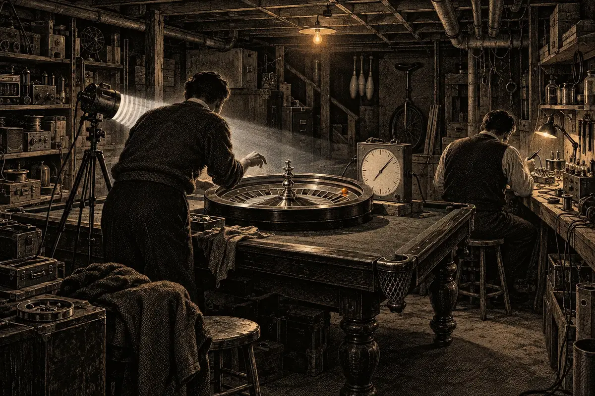
In his 1998 account, Edward Thorp dates the idea to 1955 and describes working with Claude Shannon at MIT in 1960–61. They studied a regulation wheel on a slate billiard table in Shannon’s basement, using a clock and strobe light to improve their timing.
By June 1961 they had a cigarette-pack-sized analog computer with twelve transistors. Toe-operated switches timed the ballꯈꯨꯠꯂꯥꯏꯕꯣꯜꯔꯣꯇꯔꯒꯤ ꯃꯥꯌꯣꯛꯇ ꯇ꯭ꯔꯦꯛꯇ ꯊꯥꯗꯣꯛꯄ ꯑꯄꯤꯛꯄ ꯕꯣꯜ꯫ ꯍꯧꯖꯤꯛꯀꯤ ꯕꯣꯜꯁꯤꯡ ꯑꯥꯏꯚꯣꯔꯤꯟ ꯅꯠꯔꯒ ꯇꯦꯐ꯭ꯂꯣꯅꯅ ꯁꯦꯝꯃꯤ, 18–21 mm꯫ꯃꯄꯨꯡ ꯄꯥꯕꯤꯌꯨ → and rotorꯈꯨꯠꯂꯥꯏꯔꯣꯇꯔꯄꯣꯀꯦꯠꯁꯤꯡ ꯄꯨꯔꯛꯄ ꯆꯛꯔꯒꯤ ꯀꯣꯏꯕ ꯁꯔꯨꯛ꯫ꯃꯄꯨꯡ ꯄꯥꯕꯤꯌꯨ →; tones identified one of eight sectorsꯆꯛꯔꯁꯦꯛꯇꯔꯆꯛꯔꯗ ꯃꯔꯛ ꯂꯩꯇꯅ ꯃꯈꯥ ꯆꯠꯅꯅ ꯂꯩꯕ ꯄꯣꯀꯦꯠꯁꯤꯡꯒꯤ ꯁꯔꯨꯛ, ꯂꯦꯑꯥꯎꯠꯇ ꯂꯩꯕ ꯀꯥꯡꯂꯨꯞ ꯑꯃꯗꯒꯤ ꯇꯣꯉꯥꯟꯅ꯫ꯃꯄꯨꯡ ꯄꯥꯕꯤꯌꯨ → to bet on. Thorp reports testing it in Las Vegas that summer with ten-cent chipsꯁꯦꯜꯆꯤꯞꯂꯦꯞꯂꯕ ꯁꯦꯜꯒꯤ ꯃꯃꯜ ꯇꯥꯛꯄ ꯇꯣꯀꯟ, ꯕꯦꯠ ꯊꯝꯅꯕ ꯂꯦꯑꯥꯎꯠꯇ ꯊꯝꯃꯤ꯫ ꯑꯇꯣꯞꯄ ꯃꯃꯤꯡ: ꯆꯦꯛ꯫ꯃꯄꯨꯡ ꯄꯥꯕꯤꯌꯨ →. Repeated breaks in the earpiece wires prevented sustained serious betting. Distance and competing work later kept the project from continuing.
This is the inventor’s retrospective account, not an independent casino trial report. His 1969 paper gives 1957 for the initial idea; the later account gives 1955. Both describe work completed by 1961.
ꯑꯍꯥꯅꯕ ꯗꯤꯖꯤꯇꯦꯜ ꯀꯝꯄꯤꯎꯇꯔꯁꯤꯡ
ꯊꯣꯔꯞ ꯑꯃꯁꯨꯡ ꯁꯦꯅꯟꯒꯤ ꯃꯦꯁꯤꯟ ꯑꯁꯤ ꯑꯦꯅꯥꯂꯣꯒꯅꯤ: ꯃꯁꯤꯒꯤ ꯁꯔꯀꯤꯠ ꯑꯁꯤꯅ ꯃꯁꯤꯒꯤ ꯄ꯭ꯔꯣꯒ꯭ꯔꯥꯃꯅꯤ, ꯑꯃꯁꯨꯡ ꯃꯑꯣꯡ ꯍꯣꯡꯗꯣꯛꯅꯕ ꯇꯥꯔ ꯑꯅꯧꯅ ꯁꯦꯝꯕ ꯃꯊꯧ ꯇꯥꯔꯝꯃꯤ꯫ ꯃꯥꯏꯛꯔꯣꯄ꯭ꯔꯣꯁꯦꯁꯔꯅ ꯉꯃꯈꯩ ꯑꯗꯨ ꯂꯧꯊꯣꯀꯈꯤ꯫ ꯀꯦꯜꯇꯦꯀꯀꯤ ꯁ꯭ꯇꯨꯗꯦꯟꯠ ꯑꯦꯂꯟ ꯂꯨꯏꯁꯅ 1972 ꯗ ꯌꯨꯃꯗ ꯁꯦꯃꯈꯤꯕ ꯗꯤꯖꯤꯇꯦꯜ ꯀꯝꯄꯤꯎꯇꯔ ꯑꯃꯥ ꯀꯦꯃꯦꯔꯥ ꯀꯦꯁ ꯑꯃꯗ ꯊꯃꯗꯨꯅ ꯂꯥꯁ ꯚꯦꯒꯥꯁꯀꯤ ꯁꯥꯔꯀꯁ ꯁꯥꯔꯀꯁꯇ ꯄꯨꯈꯤ, ꯇꯦꯕꯜꯁꯤꯡꯒꯤ ꯃꯊꯛꯇ ꯂꯩꯕ ꯕꯦꯂꯀꯣꯅꯤ ꯑꯃꯗꯒꯤ ꯆꯛꯔꯁꯤꯡꯒꯤ ꯃꯇꯝ ꯊꯥꯖꯈꯤ ꯑꯃꯁꯨꯡ ꯃꯈꯥꯗ ꯂꯩꯕ ꯃꯔꯨꯞ ꯑꯃꯗ ꯔꯦꯗꯤꯑꯣꯅ ꯂꯥꯏꯃꯥꯏ ꯁꯟꯕꯁꯤꯡ ꯊꯥꯈꯤ꯫ ꯃꯁꯤ ꯆꯠꯈꯤ, ꯑꯗꯨꯕꯨ ꯁꯦꯜ ꯑꯃꯠꯇ ꯀꯥꯟꯈꯤꯗꯦ; ꯃꯇꯨꯡꯗ ꯃꯍꯥꯛꯅ ꯆꯛꯔꯒꯤ ꯊꯣꯡꯕ ꯑꯗꯨ ꯊꯥꯗꯣꯀꯈꯤ ꯍꯥꯌꯕ ꯈꯉꯈꯤ꯫ 1976 ꯗꯒꯤ ꯁꯥꯟꯇꯥ ꯀ꯭ꯔꯨꯖꯒꯤ ꯐꯤꯖꯤꯛꯁ ꯁ꯭ꯇꯨꯗꯦꯟꯇꯁꯤꯡꯒꯤ ꯀꯥꯡꯕꯨ ꯑꯃꯥ, ꯌꯨꯗꯦꯃꯣꯅꯁꯤꯡꯅ, ꯊꯕꯛ ꯑꯁꯤ ꯃꯄꯨꯡ ꯐꯥꯅ ꯇꯧꯈꯤ꯫ ꯃꯈꯣꯌꯅ ꯀꯦꯁꯤꯅꯣꯒꯤ ꯆꯛꯔ ꯑꯃꯥ ꯂꯩꯈꯤ, ꯕꯣꯜ, ꯔꯣꯇꯔ, ꯊꯣꯡꯕ ꯑꯃꯁꯨꯡ ꯆꯣꯡꯕ ꯊꯥꯖꯈꯤ, ꯑꯃꯁꯨꯡ ꯁꯦꯇꯤꯡ ꯃꯉꯥ ꯂꯩꯕ ꯏꯀ꯭ꯕꯦꯁꯟꯁꯤꯡ ꯏꯈꯤ, ꯃꯗꯨ ꯁꯥꯟꯅꯔꯤꯕꯅ ꯕꯦꯠ ꯊꯝꯕꯒꯤ ꯃꯃꯥꯡꯗ ꯃꯤꯅꯤꯠ ꯀꯨꯟ ꯈꯟꯅꯕ ꯈꯣꯡꯒꯤ ꯁ꯭ꯋꯤꯆꯁꯤꯡ ꯅꯝꯗꯨꯅ ꯆꯛꯔ ꯈꯨꯗꯤꯡꯒꯤꯗꯃꯛ ꯁꯦꯃꯗꯣꯛ-ꯁꯦꯃꯖꯤꯟ ꯇꯧꯔꯝꯃꯤ꯫ ꯃꯈꯣꯌꯒꯤ ꯀꯝꯄꯤꯎꯇꯔꯅ ꯁ꯭ꯄꯤꯟ ꯍꯧꯔꯕꯥ ꯆꯦꯛꯀꯟꯗ ꯈꯔꯒꯤ ꯃꯇꯨꯡꯗ ꯁꯦꯛꯇꯔ ꯅꯤꯄꯥꯟꯒꯤ ꯑꯃꯒꯤ ꯃꯃꯤꯡ ꯍꯥꯌꯔꯝꯃꯤ꯫ ꯖꯥꯅꯨꯋꯥꯔꯤ 1978 ꯗ ꯑꯁꯦꯡꯕ ꯇꯦꯕꯜ ꯑꯃꯗ ꯃꯁꯤꯅ ꯃꯈꯣꯌꯅ 25% ꯍꯥꯌꯅ ꯈꯟꯅꯈꯤꯕ ꯑꯦꯖ ꯑꯃꯥ ꯄꯤꯈꯤ; ꯍꯛꯆꯥꯡꯗ ꯊꯃꯖꯤꯜꯂꯕ ꯑꯃꯁꯨꯡ ꯃꯇꯨꯡꯗ ꯈꯣꯡꯎꯞꯇ ꯁꯦꯝꯕ ꯍꯥꯔꯗꯋꯦꯌꯔ ꯑꯗꯨ ꯐꯤꯖꯤꯛꯁꯇꯒꯤ ꯌꯥꯝꯅ ꯍꯦꯟꯅꯥ ꯃꯇꯝ ꯀꯌꯥꯗ ꯐꯦꯜ ꯇꯧꯈꯤ (ꯌꯨꯗꯦꯃꯣꯅꯁꯤꯡ ꯌꯦꯡꯕꯤꯌꯨ)꯫
ꯃꯇꯨꯡꯗ ꯊꯝꯕ ꯕꯦꯠꯁꯤꯡ ꯀꯔꯤꯒꯤ ꯃꯔꯨꯑꯣꯏꯈꯤꯕꯒꯦ
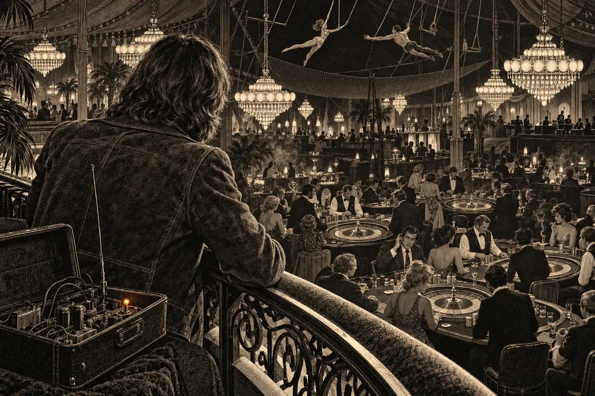
A strategy that measures the current spin cannot use those measurements if betting has already closed. Thorp’s account describes late betting in games he observed, not every modern studio. Nevada’s device provision dates to 1985; its current wording includes an approval exception.
ꯀꯦꯁꯤꯅꯣꯁꯤꯡꯅ ꯀꯔꯝꯅ ꯂꯥꯟꯊꯦꯡꯅꯈꯤꯕꯒꯦ
A predictor fitted to one setup needs fresh validation when the wheel, ball or operating conditions change. A change does not by itself prove that prediction has become impossible; what matters is the resulting prediction error and whether it still supports the proposed bet.
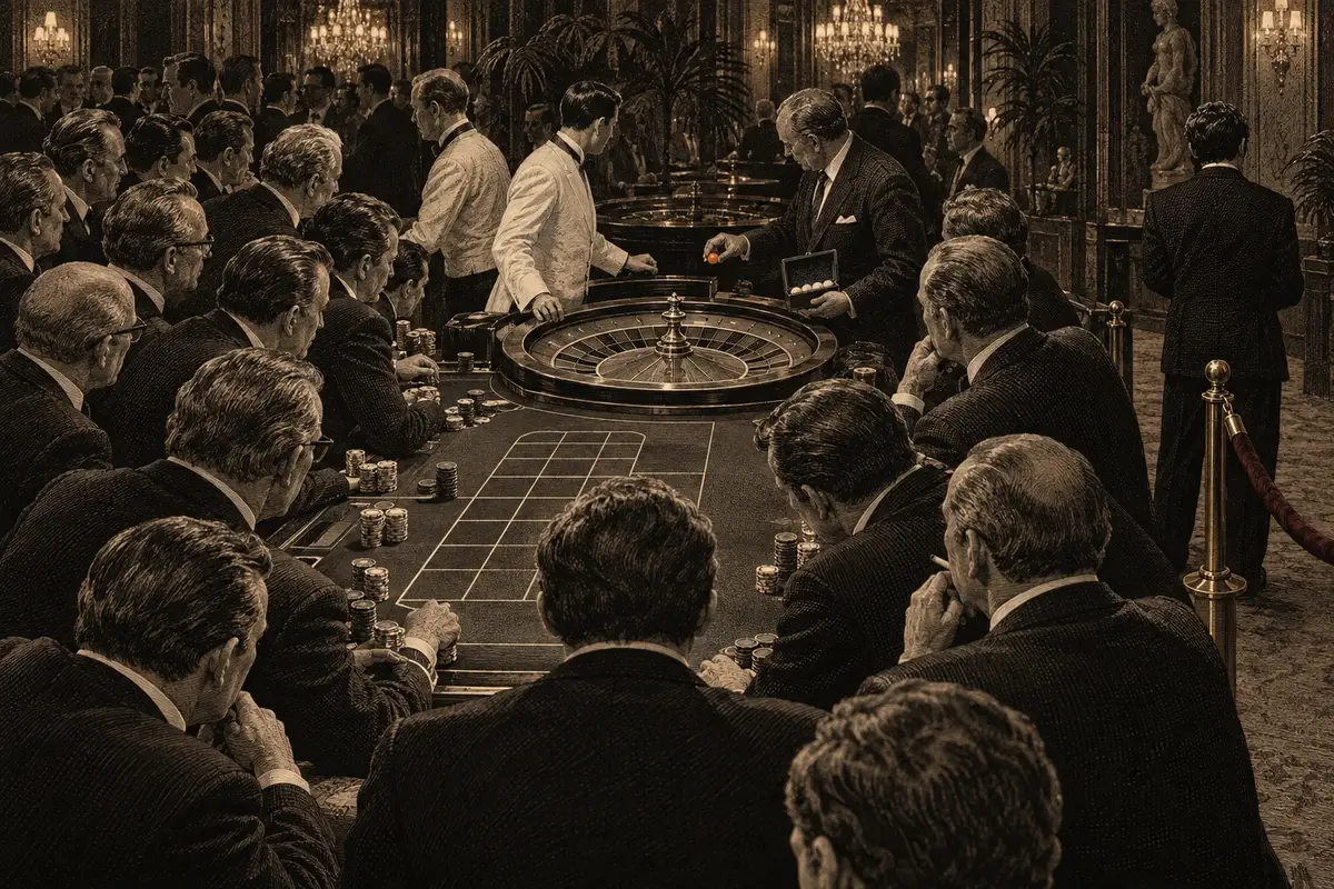
In his 1998 account, Thorp identifies closing bets before launch as a way to prevent his method from using the current spin. This is a constraint on that method, not evidence that every casino follows the same procedure. Check the actual betting deadline rather than assuming that a historical account describes today’s game.
ꯂꯥꯏꯃꯥꯏ ꯁꯟꯕ ꯀꯌꯥ ꯐꯒꯗꯒꯦ
The table uses a mathematical model: prediction error is a centered normal distribution wrapped around 37 pocketsꯈꯨꯠꯂꯥꯏꯄꯣꯀꯦꯠꯔꯣꯇꯔꯗ ꯂꯩꯕ ꯃꯁꯤꯡ ꯏꯔꯕ ꯀꯣꯠ 37 ꯒꯤ ꯃꯅꯨꯡꯗ ꯑꯃꯥ꯫ ꯑꯇꯣꯞꯄ ꯃꯃꯤꯡ: ꯁ꯭ꯂꯣꯠ, ꯀꯞ꯫ꯃꯄꯨꯡ ꯄꯥꯕꯤꯌꯨ →, each one unitꯁꯦꯜꯌꯨꯅꯤꯠꯁꯤꯁ꯭ꯇꯦꯝ ꯅꯠꯔꯒ ꯁꯥꯟꯅꯔꯤꯕ ꯑꯃꯅ ꯁꯤꯖꯤꯟꯅꯕ ꯃꯔꯨꯑꯣꯏꯕ ꯊꯝꯂꯕ ꯁꯦꯜ꯫ ꯄ꯭ꯔꯣꯒ꯭ꯔꯦꯁꯅꯁꯤꯡ ꯌꯨꯅꯤꯠꯇ ꯁꯟꯗꯣꯛꯂꯤ, ꯃꯔꯝ ꯑꯗꯨꯅ ꯃꯈꯣꯌ ꯀꯔꯤꯒꯨꯝꯕ ꯇꯦꯕꯜꯗ ꯆꯠꯂꯤ꯫ꯃꯄꯨꯡ ꯄꯥꯕꯤꯌꯨ → wide. Expected return follows by integrating the selected pocket interval and applying 35:1 payoutsꯁꯦꯜꯄꯦꯑꯥꯎꯠꯃꯥꯏꯄꯥꯛꯄ ꯕꯦꯠ ꯑꯃꯅ ꯍꯜꯂꯛꯄ ꯁꯦꯜ, ꯍꯜꯂꯀꯄ ꯊꯝꯂꯕ ꯁꯦꯜꯒꯤ ꯃꯊꯛꯇ “X ꯗꯒꯤ 1” ꯍꯥꯌꯅ ꯍꯥꯌꯏ꯫ꯃꯄꯨꯡ ꯄꯥꯕꯤꯌꯨ →. This is a model illustration, not measured accuracy for a current device. At σ = 10 it gives about +43.9% for one pocket or +42.5% for five centered pockets. Break-evenꯃꯦꯊꯃꯦꯇꯤꯛꯁꯕ꯭ꯔꯦꯛ-ꯏꯚꯟꯕꯦꯠ ꯑꯃꯒꯤ ꯐꯪꯒꯗꯕ ꯃꯃꯜ ꯆꯨꯃꯊꯣꯛꯅ ꯖꯤꯔꯣ ꯑꯣꯏꯕ ꯃꯐꯝ, ꯃꯔꯝ ꯑꯗꯨꯅ ꯀꯅꯥꯒꯨꯝꯕ ꯃꯥꯏꯀꯩ ꯑꯃꯠꯇꯗ ꯑꯦꯖ ꯂꯩꯇꯦ꯫ ꯌꯥꯝꯅ ꯄꯦꯑꯥꯎꯠ ꯑꯃ ꯅꯠꯔꯒ ꯖꯦꯀꯄꯣꯠꯀꯤ ꯆꯥꯎꯕ ꯑꯃꯅꯤ꯫ꯃꯄꯨꯡ ꯄꯥꯕꯤꯌꯨ → is about 17.22 pockets for one and 17.16 for five. A different error distribution gives different values.
ꯋꯥꯍꯪꯁꯤꯡ
ꯌꯥꯔꯣꯏ꯫ ꯕꯣꯜ ꯂꯩꯇꯦ꯫ ꯃꯁꯤꯡ ꯑꯗꯨ ꯑꯦꯅꯤꯃꯦꯁꯅꯒꯤ ꯃꯃꯥꯡꯗ ꯁꯣꯐꯇꯋꯦꯌꯔꯅ ꯂꯧꯊꯣꯀꯏ꯫
ꯃꯈꯣꯌꯗ ꯃꯇꯝ ꯊꯥꯖꯕꯒꯤ ꯈꯨꯗꯣꯡꯊꯤꯕ ꯂꯩꯒꯅꯤ, ꯃꯔꯝ ꯑꯗꯨꯅ ꯃꯑꯣꯡ ꯑꯗꯨꯗ ꯑꯃꯠꯇ ꯆꯂꯥꯏꯗꯦ꯫
ꯃꯦꯊꯃꯦꯇꯤꯛꯁꯀꯥ ꯁꯥꯟꯅꯕ
ꯃꯁꯤꯁꯤꯡ ꯑꯍꯥꯅꯕꯗ ꯅꯍꯥꯛ ꯃꯁꯥꯃꯛꯅ ꯍꯣꯠꯅꯕꯤꯌꯨ꯫ ꯄꯥꯎꯈꯨꯝ ꯈꯨꯗꯤꯡꯃꯛ ꯊꯨꯡꯗꯨꯅ ꯊꯝꯂꯤ; ꯁꯦꯝ ꯁꯥꯔꯕ ꯃꯇꯃꯗ ꯍꯥꯡꯗꯣꯛꯄꯤꯌꯨ꯫
ꯌꯨꯝꯂꯣꯟꯅꯕꯕꯦꯠꯌꯨꯝꯂꯣꯟꯅꯕ ꯕꯦꯠꯆꯛꯔꯗ ꯃꯁꯤꯡ ꯑꯃꯥ ꯑꯃꯁꯨꯡ ꯃꯗꯨꯒꯤ ꯅꯥꯀꯜ ꯑꯅꯤꯃꯛꯇ ꯂꯩꯕ ꯄꯣꯀꯦꯠ ꯑꯅꯤ ꯑꯅꯤ, ꯁ꯭ꯇ꯭ꯔꯦꯠ-ꯑꯞ ꯆꯤꯞ ꯃꯉꯥ꯫ꯃꯄꯨꯡ ꯄꯥꯕꯤꯌꯨ → ꯀꯣꯜ ꯑꯃꯅ ꯃꯁꯤꯡ ꯑꯃꯗ ꯑꯃꯁꯨꯡ ꯆꯛꯔꯗ ꯃꯁꯤꯒꯤ ꯃꯥꯏꯀꯩ ꯑꯅꯤꯃꯛꯇ ꯂꯩꯕ ꯄꯣꯀꯦꯠꯈꯨꯠꯂꯥꯏꯄꯣꯀꯦꯠꯔꯣꯇꯔꯗ ꯂꯩꯕ ꯃꯁꯤꯡ ꯏꯔꯕ ꯀꯣꯠ 37 ꯒꯤ ꯃꯅꯨꯡꯗ ꯑꯃꯥ꯫ ꯑꯇꯣꯞꯄ ꯃꯃꯤꯡ: ꯁ꯭ꯂꯣꯠ, ꯀꯞ꯫ꯃꯄꯨꯡ ꯄꯥꯕꯤꯌꯨ → ꯑꯅꯤ ꯑꯅꯤꯗ ꯆꯤꯞꯁꯦꯜꯆꯤꯞꯂꯦꯞꯂꯕ ꯁꯦꯜꯒꯤ ꯃꯃꯜ ꯇꯥꯛꯄ ꯇꯣꯀꯟ, ꯕꯦꯠ ꯊꯝꯅꯕ ꯂꯦꯑꯥꯎꯠꯇ ꯊꯝꯃꯤ꯫ ꯑꯇꯣꯞꯄ ꯃꯃꯤꯡ: ꯆꯦꯛ꯫ꯃꯄꯨꯡ ꯄꯥꯕꯤꯌꯨ → ꯑꯃꯃꯛ ꯊꯝꯏ: ꯆꯤꯞ ꯃꯉꯥ꯫ ꯕ꯭ꯔꯦꯛ-ꯏꯚꯟ ꯑꯣꯏꯅꯕ ꯄ꯭ꯔꯤꯗꯤꯛꯁꯟ ꯑꯃꯅ ꯄꯣꯀꯦꯠ ꯃꯉꯥ ꯑꯗꯨꯗ ꯀꯌꯥ ꯌꯥꯃꯅ ꯆꯨꯛꯀꯗꯒꯦ, ꯑꯃꯁꯨꯡ ꯃꯉꯥꯗ ꯑꯃꯨꯛ ꯆꯨꯝꯂꯕꯗꯤ ꯀꯌꯥ ꯐꯪꯒꯅꯤ?
ꯄꯥꯎꯈꯨꯝ ꯎꯠꯄ
ꯄꯥꯎꯈꯨꯝ 36 ꯗ 5, 13.9% ꯗ ꯕ꯭ꯔꯦꯛ-ꯏꯚꯟ ꯑꯣꯏ, ꯂꯥꯛꯀꯤ ꯃꯍꯩꯈꯛꯀꯤ 13.5% ꯒꯥ ꯆꯥꯡꯗꯝꯂꯕꯗ꯫ ꯃꯉꯥꯗ ꯑꯃꯨꯛ ꯆꯨꯝꯂꯕꯗꯤ, ꯊꯝꯂꯕꯗꯒꯤ 44% ꯍꯦꯟꯅ ꯍꯜꯂꯛꯏ꯫
If the call hits, one chip wins 35 to 1 and comes back with its winnings, 36 chips, and the other four are lost. So a hit returns 36 for 5 staked, and the call breaks even if it hits 5 times in 36, 13.9%. By chance it hits 5 times in 37, 13.5%. That small gap, less than half a percentage point, is where the whole 2.70% comes from.
At one hit in five, 0.2 × 36 = 7.2 chips come back for every 5 staked, +44%. At one in four, +80%.
These are expected returns under the stated success probabilities and payoutsꯁꯦꯜꯄꯦꯑꯥꯎꯠꯃꯥꯏꯄꯥꯛꯄ ꯕꯦꯠ ꯑꯃꯅ ꯍꯜꯂꯛꯄ ꯁꯦꯜ, ꯍꯜꯂꯀꯄ ꯊꯝꯂꯕ ꯁꯦꯜꯒꯤ ꯃꯊꯛꯇ “X ꯗꯒꯤ 1” ꯍꯥꯌꯅ ꯍꯥꯌꯏ꯫ꯃꯄꯨꯡ ꯄꯥꯕꯤꯌꯨ →. A prediction would need independently measured accuracy; this calculation does not establish that any device or player achieves it.
Consider four independent, zeroꯆꯛꯔꯖꯤꯔꯣꯆꯞ ꯃꯥꯟꯅꯕ, ꯗꯖꯟ ꯅꯠꯔꯒ ꯀꯂꯝ ꯕꯦꯠ ꯑꯃꯠꯇꯅ ꯀꯨꯞꯇꯕ ꯑꯁꯪꯕ ꯄꯣꯀꯦꯠ ꯑꯃꯈꯛꯇ; ꯍꯥꯎꯁ ꯑꯦꯖꯀꯤ ꯍꯧꯔꯀꯐꯝꯅꯤ꯫ ꯑꯇꯣꯞꯄ ꯃꯃꯤꯡ: ꯁꯤꯡꯒꯜ ꯖꯤꯔꯣ, 0꯫ꯃꯄꯨꯡ ꯄꯥꯕꯤꯌꯨ →-mean prediction errors whose standard deviationsꯃꯦꯊꯃꯦꯇꯤꯛꯁꯁ꯭ꯇꯦꯟꯗꯔꯗ ꯗꯤꯚꯤꯌꯦꯁꯟꯚꯦꯌꯔꯤꯌꯦꯟꯁꯀꯤ ꯁ꯭ꯀ꯭ꯋꯦꯌꯔ ꯔꯨꯠ; ꯃꯍꯩ ꯑꯃꯅ ꯐꯪꯒꯗꯕ ꯃꯃꯜꯗꯒꯤ ꯌꯥꯝꯅ ꯂꯥꯞꯄ ꯃꯑꯣꯡ꯫ꯃꯄꯨꯡ ꯄꯥꯕꯤꯌꯨ →, measured in pockets, are 1.4, 5.5, 7 and 6. The first two represent timing errors. What is the combined standard deviation, and how much would eliminating both timing errors reduce it?
ꯄꯥꯎꯈꯨꯝ ꯎꯠꯄ
ꯄꯥꯎꯈꯨꯝ ꯄꯨꯝꯅꯃꯛ ꯄꯣꯀꯦꯠ 10.8 ꯈꯔ꯫ ꯃꯇꯝ ꯂꯦꯞꯄꯒꯤ ꯑꯔꯥꯟꯕꯁꯤꯡ ꯌꯥꯎꯗꯔꯕꯗꯤ 9.2 ꯑꯣꯏꯒꯅꯤ, ꯃꯔꯝ ꯑꯗꯨꯅ ꯃꯇꯝ ꯂꯦꯞꯄ ꯑꯅꯤꯅ 1.6 ꯈꯛ ꯍꯥꯄꯆꯤꯜꯂꯤ꯫
For independent errors, variancesꯃꯦꯊꯃꯦꯇꯤꯛꯁꯚꯦꯌꯔꯤꯌꯦꯟꯁꯃꯍꯩꯁꯤꯡ ꯐꯪꯒꯗꯕ ꯃꯃꯂꯒꯤ ꯑꯀꯣꯌꯕꯗ ꯀꯌꯥ ꯁꯟꯗꯣꯛꯅ ꯂꯩꯕꯒꯦ ꯍꯥꯌꯕꯒꯤ ꯆꯥꯡ꯫ ꯁ꯭ꯇ꯭ꯔꯦꯠ-ꯑꯞꯇ ꯋꯥꯡꯏ, ꯆꯞ ꯃꯥꯟꯅꯕ ꯕꯦꯠꯁꯤꯡꯗ ꯅꯦꯝꯏ꯫ꯃꯄꯨꯡ ꯄꯥꯕꯤꯌꯨ → add. The combined standard deviation is √(1.4² + 5.5² + 7² + 6²) = √117.21 ≈ 10.83 pockets.
Without the timing errors it is √(7² + 6²) = √85 ≈ 9.22 pockets. The reduction is about 1.61 pockets, not 1.4 + 5.5.
This is a hypothetical error budget. Correlated errors require covariance terms, and a standard deviation alone does not determine a prediction’s hit rate or betting return.
ꯅꯣꯛꯅꯕꯒꯤ ꯀꯃꯤꯛ
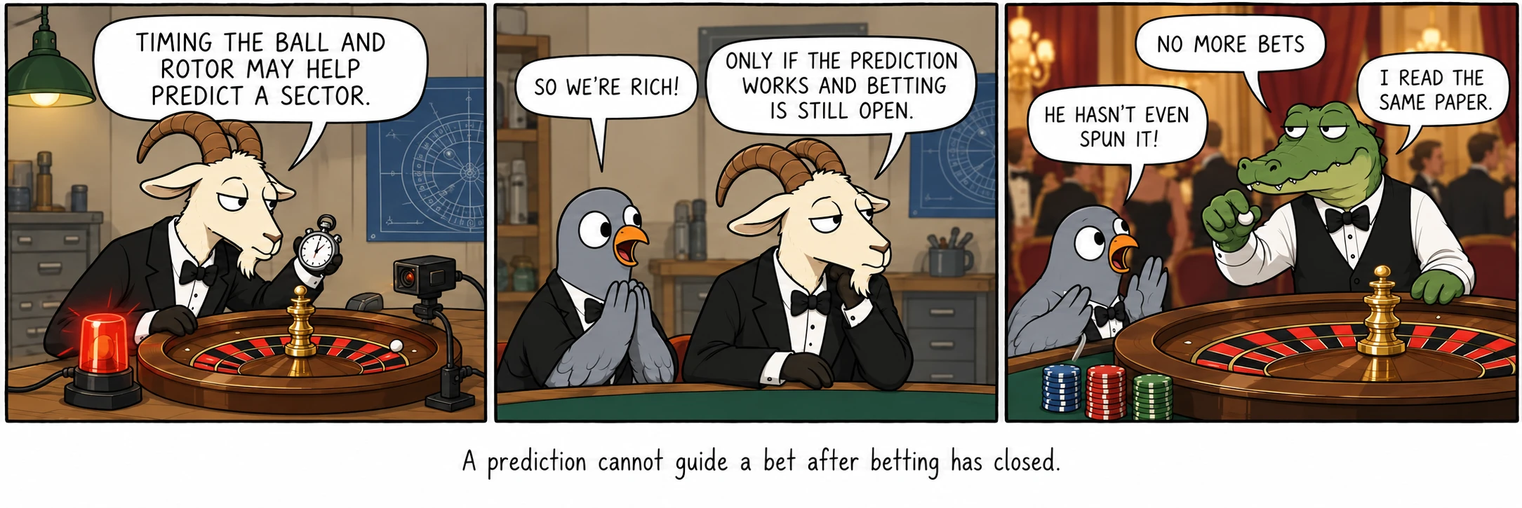
ꯐꯤꯖꯤꯛꯁ ꯊꯕꯛ ꯇꯧꯏ꯫ ꯕꯦꯠ ꯊꯝꯕꯒꯤ ꯃꯇꯝ ꯊꯤꯡꯖꯤꯜꯂꯦ꯫
ꯍꯧꯔꯛꯐꯃꯁꯤꯡ
- Thorp, E. O. “Optimal gambling systems for favorable games.”
- Thorp, E. O. The Mathematics of Gambling.
- Thorp, E. O. “The invention of the first wearable computer.”
- Bass, T. A. The Eudaemonic Pie.
- Small, M. & Tse, C. K. “Predicting the outcome of roulette.”
- Goldman, N. Great Gambling Scams.
- Nevada Revised Statutes, chapter 465.
- Edward O. Thorp, The Invention of the First Wearable Computer
- Nevada Revised Statutes 465.075 — 2026ꯒꯤ ꯅꯣꯚꯦꯝꯕꯔ 15ꯗ ꯌꯦꯡꯁꯤꯟꯈꯤ
- Bradley Rhodes, A brief history of wearable computing
- J. Doyne Farmer, Roulette
- Heinz Nixdorf MuseumsForum, Shoe computer