ꯀꯦꯂꯤ ꯀ꯭ꯔꯥꯏꯇꯦꯔꯤꯌꯟ ꯑꯃꯁꯨꯡ ꯔꯨꯂꯦꯠ
ꯀꯦꯂꯤ ꯀ꯭ꯔꯥꯏꯇꯦꯔꯤꯌꯟꯅ ꯑꯦꯖ ꯂꯩꯕ ꯕꯦꯠ ꯊꯝꯕ ꯃꯤ ꯑꯃꯕꯨ ꯀꯌꯥ ꯊꯝꯒꯗꯒꯦ ꯍꯥꯌꯕ ꯇꯥꯀꯏ꯫ ꯔꯨꯂꯦꯠꯀꯤꯗꯃꯛ ꯃꯁꯤꯅ ꯃꯌꯦꯛ ꯁꯦꯡꯕ ꯄꯥꯎꯈꯨꯝ ꯑꯃꯥ ꯄꯤꯔꯤ: ꯀꯔꯤꯒꯨꯝꯕ ꯑꯃꯠꯇ ꯊꯝꯒꯅꯨ꯫

ꯀꯦꯂꯤ ꯊꯝꯂꯕ ꯁꯦꯜ = ꯑꯦꯖ / ꯑꯣꯗꯁ꯫ ꯑꯦꯖ ꯑꯗꯨ ꯅꯦꯒꯦꯇꯤꯕ ꯑꯣꯏꯔꯕꯗꯤ ꯐꯣꯔꯃꯨꯂꯥ ꯑꯁꯤꯅ ꯅꯦꯒꯦꯇꯤꯕ ꯁꯔꯨꯛ ꯑꯃꯥ ꯄꯤꯔꯤ, ꯃꯁꯤꯒꯤ ꯑꯔꯊꯗꯤ ꯕꯦꯠ ꯊꯝꯒꯅꯨ꯫ ꯕꯥꯏꯌꯥꯁ ꯁꯥꯟꯅꯔꯤꯕꯁꯤꯡꯅ ꯃꯈꯣꯌꯒꯤ ꯕꯦꯠꯀꯤ ꯆꯥꯡ ꯀꯔꯤꯒꯤ ꯃꯇꯧ ꯑꯗꯨꯒꯨꯝꯅ ꯂꯦꯞꯈꯤꯕꯒꯦ, ꯑꯃꯁꯨꯡ ꯑꯇꯩ ꯄꯨꯝꯅꯃꯛꯅ ꯀꯔꯤꯒꯤ ꯕꯖꯦꯠꯀꯤ ꯃꯇꯨꯡ ꯏꯟꯅ ꯆꯥꯡ ꯂꯦꯞꯀꯗꯒꯦ ꯍꯥꯌꯕ ꯈꯉꯅꯕꯗ ꯀ꯭ꯔꯥꯏꯇꯦꯔꯤꯌꯟ ꯑꯁꯤ ꯍꯧꯖꯤꯀꯁꯨ ꯀꯥꯟꯅꯩ꯫
ꯀ꯭ꯔꯥꯏꯇꯦꯔꯤꯌꯟ
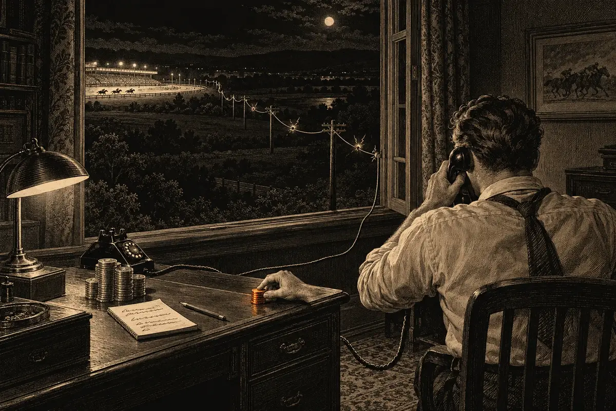
John Kelly (1956) asked how a gambler with a known edge should size bets to maximize long-run growth of the bankrollꯁꯦꯜꯕꯦꯡꯀꯔꯣꯜꯁꯥꯟꯅꯅꯕ ꯇꯣꯉꯥꯟꯅ ꯊꯝꯂꯕ ꯁꯦꯜ ꯄꯨꯝꯅꯃꯛ꯫ ꯕꯦꯡꯀꯔꯣꯜ ꯃꯦꯅꯦꯖꯃꯦꯟꯠ ꯍꯥꯌꯕꯁꯤ ꯃꯗꯨꯒꯤ ꯀꯌꯥ ꯕꯦꯠ ꯈꯨꯗꯤꯡꯗ ꯑꯃꯁꯨꯡ ꯁꯦꯁꯟ ꯈꯨꯗꯤꯡꯗ ꯈꯨꯗꯣꯡꯊꯤꯕꯗ ꯊꯃꯒꯗꯒꯦ ꯍꯥꯌꯕ ꯋꯥꯔꯦꯞ ꯂꯧꯕꯅꯤ꯫ꯃꯄꯨꯡ ꯄꯥꯕꯤꯌꯨ →. The answer, for a bet paying b to 1 with win probabilityꯃꯦꯊꯃꯦꯇꯤꯛꯁꯊꯣꯛꯄꯒꯤ ꯈꯨꯗꯣꯡꯆꯥꯕꯃꯍꯩ ꯑꯃꯥ ꯊꯣꯛꯄꯒꯤ ꯈꯨꯗꯣꯡꯆꯥꯕ, 0 ꯗꯒꯤ 1 ꯐꯥꯑꯣꯕ ꯅꯠꯔꯒ 0% ꯗꯒꯤ 100% ꯐꯥꯑꯣꯕ꯫ ꯃꯁꯤꯡ ꯑꯃꯥ: 1/37 = 2.70%꯫ꯃꯄꯨꯡ ꯄꯥꯕꯤꯌꯨ → p and loss probability q = 1 − p, is to stake the fraction f* = (bp − q) / b of the bankroll. Positive f* means bet that fraction; zero or negative means do not bet. Kelly worked at Bell Labs, and his paper, “A new interpretation of information rate”, set the problem in Claude Shannon’s theory of information: a gambler who gets tips over a noisy line, at fair odds, can grow the bankroll at best at the rate the line carries information. This is a growth objective under a probability model, not a promise to finish ahead after a particular number of bets. A spending limit, finite deadline or payoutꯁꯦꯜꯄꯦꯑꯥꯎꯠꯃꯥꯏꯄꯥꯛꯄ ꯕꯦꯠ ꯑꯃꯅ ꯍꯜꯂꯛꯄ ꯁꯦꯜ, ꯍꯜꯂꯀꯄ ꯊꯝꯂꯕ ꯁꯦꯜꯒꯤ ꯃꯊꯛꯇ “X ꯗꯒꯤ 1” ꯍꯥꯌꯅ ꯍꯥꯌꯏ꯫ꯃꯄꯨꯡ ꯄꯥꯕꯤꯌꯨ → cap changes the decision problem.
ꯔꯨꯂꯦꯠꯇ ꯀꯦꯂꯤ ꯕꯦꯇꯤꯡ
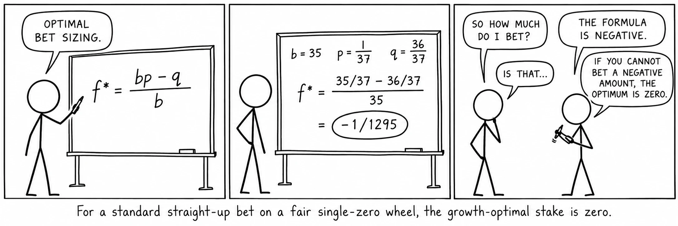
For redꯕꯦꯠꯑꯉꯥꯡꯕꯑꯉꯥꯡꯕ ꯃꯁꯤꯡ 18 ꯗ ꯊꯝꯕ ꯆꯞ ꯃꯥꯟꯅꯕ ꯕꯦꯠ꯫ ꯐ꯭ꯔꯦꯟꯆ: ꯔꯨꯖ꯫ꯃꯄꯨꯡ ꯄꯥꯕꯤꯌꯨ →: b = 1, p = 18/37, q = 19/37; f* = (18/37 − 19/37)/1 = −1/37. For a straight upꯕꯦꯠꯁ꯭ꯇ꯭ꯔꯦꯠ-ꯑꯞꯃꯁꯤꯡ ꯑꯃꯈꯛꯇ, 35:1 ꯄꯦꯑꯥꯎꯠ꯫ꯃꯄꯨꯡ ꯄꯥꯕꯤꯌꯨ →: b = 35, p = 1/37, q = 36/37; f* = (35/37 − 36/37)/35 = −1/1295. Every standard bet gives a negative Kelly fraction, because every bet has a negative edge, and the growth-optimal stake is zero. Kelly betting on roulette is a formal way of saying what the house-edge page says: no positive stake maximizes expected logarithmic growth when the bet has negative expectation. A particular session can still end in profit. La partageꯅꯤꯌꯝꯂꯥ ꯄꯥꯔꯇꯥꯖꯐ꯭ꯔꯦꯟꯆ ꯅꯤꯌꯝ: ꯖꯤꯔꯣ ꯊꯣꯛꯂꯕꯗꯤ ꯆꯞ ꯃꯥꯟꯅꯕ ꯕꯦꯠꯀꯤ ꯊꯝꯂꯕ ꯁꯦꯜꯒꯤ ꯁꯔꯨꯛ ꯑꯍꯦꯟꯕ ꯍꯜꯂꯀꯏ꯫ ꯕꯦꯠ ꯑꯗꯨꯁꯤꯡꯒꯤ ꯍꯥꯎꯁ ꯑꯦꯖ 1.35% ꯐꯥꯑꯣꯕ ꯁꯔꯨꯛ ꯑꯅꯤꯗ ꯊꯥꯖꯤꯜꯂꯤ꯫ꯃꯄꯨꯡ ꯄꯥꯕꯤꯌꯨ → needs a separate three-outcome calculation: a win, a full loss or a half-loss on zeroꯆꯛꯔꯖꯤꯔꯣꯆꯞ ꯃꯥꯟꯅꯕ, ꯗꯖꯟ ꯅꯠꯔꯒ ꯀꯂꯝ ꯕꯦꯠ ꯑꯃꯠꯇꯅ ꯀꯨꯞꯇꯕ ꯑꯁꯪꯕ ꯄꯣꯀꯦꯠ ꯑꯃꯈꯛꯇ; ꯍꯥꯎꯁ ꯑꯦꯖꯀꯤ ꯍꯧꯔꯀꯐꯝꯅꯤ꯫ ꯑꯇꯣꯞꯄ ꯃꯃꯤꯡ: ꯁꯤꯡꯒꯜ ꯖꯤꯔꯣ, 0꯫ꯃꯄꯨꯡ ꯄꯥꯕꯤꯌꯨ →. Its expected log growth also falls as the stake increases from zero.
ꯀꯦꯂꯤ ꯀꯗꯥꯏꯗ ꯁꯤꯖꯤꯟꯅꯈꯤꯕꯒꯦ
Suppose a pocketꯈꯨꯠꯂꯥꯏꯄꯣꯀꯦꯠꯔꯣꯇꯔꯗ ꯂꯩꯕ ꯃꯁꯤꯡ ꯏꯔꯕ ꯀꯣꯠ 37 ꯒꯤ ꯃꯅꯨꯡꯗ ꯑꯃꯥ꯫ ꯑꯇꯣꯞꯄ ꯃꯃꯤꯡ: ꯁ꯭ꯂꯣꯠ, ꯀꯞ꯫ꯃꯄꯨꯡ ꯄꯥꯕꯤꯌꯨ → really has a stable, known probability of 1 in 30 and pays 35 to 1. The Kelly fraction is 0.57%: about $57 from a $10,000 bankroll. Under independent spinsꯃꯦꯊꯃꯦꯇꯤꯛꯁꯃꯔꯤ ꯂꯩꯅꯗꯕ ꯁ꯭ꯄꯤꯟꯁꯤꯡꯍꯥꯟꯅꯒꯤ ꯃꯍꯩ ꯀꯔꯤꯒꯨꯝꯕ ꯑꯣꯏꯔꯕꯁꯨ ꯁ꯭ꯄꯤꯟ ꯈꯨꯗꯤꯡꯃꯛꯀꯤ ꯊꯣꯛꯄꯒꯤ ꯈꯨꯗꯣꯡꯆꯥꯕ ꯃꯥꯟꯅꯩ꯫ ꯋꯦꯕꯁꯥꯏꯠ ꯑꯁꯤꯒꯤ ꯊꯤꯕ ꯈꯨꯗꯤꯡꯃꯛꯀꯤ ꯌꯨꯝꯐꯝꯅꯤ꯫ꯃꯄꯨꯡ ꯄꯥꯕꯤꯌꯨ → and exact fractional staking, the geometric growth factor over 1,000 spins is about 1.7. Expected bankroll grows faster because rare large wins pull up the average. These are model calculations, not evidence that any named historical player used Kelly or achieved this result.
ꯑꯣꯏꯕ ꯃꯑꯣꯡ ꯑꯃꯁꯨꯡ ꯑꯦꯚꯔꯦꯖ
The gap between the typical bankroll and the average one is wide. Take a pocket that hits 1 time in 25, a hypothetical edge of 44% per unitꯁꯦꯜꯌꯨꯅꯤꯠꯁꯤꯁ꯭ꯇꯦꯝ ꯅꯠꯔꯒ ꯁꯥꯟꯅꯔꯤꯕ ꯑꯃꯅ ꯁꯤꯖꯤꯟꯅꯕ ꯃꯔꯨꯑꯣꯏꯕ ꯊꯝꯂꯕ ꯁꯦꯜ꯫ ꯄ꯭ꯔꯣꯒ꯭ꯔꯦꯁꯅꯁꯤꯡ ꯌꯨꯅꯤꯠꯇ ꯁꯟꯗꯣꯛꯂꯤ, ꯃꯔꯝ ꯑꯗꯨꯅ ꯃꯈꯣꯌ ꯀꯔꯤꯒꯨꯝꯕ ꯇꯦꯕꯜꯗ ꯆꯠꯂꯤ꯫ꯃꯄꯨꯡ ꯄꯥꯕꯤꯌꯨ → staked. Kelly stakes 1.26% of the bankroll on it. After 1,000 spins the typical bankroll has grown about 11.5 times, while the average, pulled up by a few very lucky runs, has grown about 249 times. Betting more than Kelly raises the average and lowers the typical result: at twice the Kelly stake the typical bankroll only doubles, and by two and a half times the Kelly stake it shrinks, although every bet still carries a 44% edge. In this example, half-Kelly retains about 78% of the expected log growth. This fraction depends on the probabilities and payout.
ꯑꯦꯖ ꯑꯗꯨ ꯈꯟꯖꯤꯟꯕ ꯈꯛꯇꯅꯤ ꯑꯣꯏꯔꯕꯗꯤ
Kelly uses the true probabilities, but a player usually has only estimates. Selecting the busiest pocket from a past record creates a selection problem: even a fair wheel has a busiest pocket. Its observed rate can overstate its future probability. Choosing the stake from that same record compounds the error. An independent follow-up sample helps test a proposed bias (see How to Detect Roulette Wheel Bias). Reducing the calculated fraction reduces exposure, but cannot turn a false edge into a real one.
ꯑꯦꯖ ꯂꯩꯕ ꯃꯤꯑꯣꯏꯁꯤꯡ
Haghani and Dewey (2016) studied 61 participants given $25 and 30 minutes to bet on a simulated coin with a disclosed 60% chance of heads. The payout cap was $250; its value was revealed when a proposed winning bet would reach it. Their reported 21% success category included balances of at least $200, while the 28% “bust” category meant less than $2, not necessarily zero. Eighteen participants bet their entire balance on one flip. The uncapped Kelly fraction is 20%, but the cap and deadline change the optimization problem. The experiment illustrates how stake choices matter even with a known advantage; it does not establish one best strategy for every objective.
ꯃꯗꯨꯒꯤ ꯃꯍꯨꯠꯇ ꯀꯔꯤ ꯁꯤꯖꯤꯟꯅꯒꯗꯒꯦ
ꯑꯦꯖ ꯂꯩꯇꯕꯗꯤ ꯆꯥꯡ ꯂꯦꯞꯄ ꯑꯁꯤ ꯕꯖꯦꯠꯀꯤ ꯋꯥꯍꯪꯅꯤ, ꯍꯦꯅꯒꯠꯄꯒꯤ ꯋꯥꯍꯪ ꯅꯠꯇꯦ: ꯊꯝꯂꯕ ꯁꯦꯜ = ꯅꯍꯥꯛꯅ ꯁ꯭ꯄꯤꯟ ꯈꯨꯗꯤꯡꯗ ꯁꯤꯖꯤꯟꯅꯕ ꯄꯥꯝꯂꯤꯕ ꯁꯦꯜ, ꯄꯨꯡ ꯈꯨꯗꯤꯡꯒꯤ ꯕꯖꯦꯠ ꯑꯃꯁꯨꯡ ꯇꯦꯕꯜꯒꯤ ꯊꯨꯅꯕꯗꯒꯤ ꯂꯧꯊꯣꯀꯄ (ꯕꯦꯡꯀꯔꯣꯜ ꯃꯦꯅꯦꯖꯃꯦꯟꯇꯀꯤ ꯂꯃꯥꯏ)꯫ ꯃꯤꯅꯝ ꯁꯥꯟꯅꯔꯤꯕꯗ ꯀꯦꯂꯤꯅ ꯄꯤꯕ ꯈꯨꯗꯣꯜ ꯑꯗꯨꯗꯤ ꯃꯁꯤꯒꯤ ꯄꯥꯎꯈꯨꯃꯒꯤ ꯃꯌꯦꯛ ꯁꯦꯡꯕꯅꯤ: ꯖꯤꯔꯣ꯫ ꯅꯍꯥꯛꯅ ꯖꯤꯔꯣꯗꯒꯤ ꯍꯦꯟꯅ ꯊꯝꯂꯤꯕ ꯄꯨꯝꯅꯃꯛ ꯑꯁꯤ ꯁꯥꯟꯅꯕꯒꯤ ꯃꯃꯂꯅꯤ, ꯅꯍꯥꯛꯅ ꯈꯅꯕ, ꯀꯔꯤꯒꯨꯝꯕ ꯐꯣꯔꯃꯨꯂꯥ ꯑꯃꯅ ꯑꯣꯞꯇꯤꯃꯥꯏꯖ ꯇꯧꯕ ꯅꯠꯇꯦ꯫
ꯁꯔꯨꯛ ꯀꯦꯂꯤ ꯑꯃꯁꯨꯡ “ꯁꯦꯜ ꯃꯦꯅꯦꯖꯃꯦꯟꯠ” ꯒꯤ ꯃꯔꯃꯗ ꯋꯥꯐꯝ ꯑꯃꯥ
Betting a fixed percentage of the current bankroll is proportional staking: the stake rises after wins and falls after losses. Flat bettingꯊꯧꯔꯥꯡꯐ꯭ꯂꯦꯠ ꯕꯦꯇꯤꯡꯁ꯭ꯄꯤꯟ ꯈꯨꯗꯤꯡꯗ ꯁꯦꯜ ꯃꯥꯟꯅꯕ ꯊꯝꯕ꯫ ꯄ꯭ꯔꯣꯒ꯭ꯔꯦꯁꯟ ꯈꯨꯗꯤꯡꯃꯛ ꯆꯥꯡꯗꯝꯅꯕ ꯃꯔꯨꯑꯣꯏꯕ ꯃꯈꯥꯌꯣꯜꯅꯤ꯫ꯃꯄꯨꯡ ꯄꯥꯕꯤꯌꯨ → instead keeps the cash stake fixed. Neither creates an edge on ordinary roulette. With infinitely divisible stakes and a fraction below 100%, proportional staking never reaches exactly zero in finitely many losses, but the balance can become arbitrarily small. Real table minimums can prevent further play much sooner. The growth-optimal fraction remains zero.
ꯐꯣꯔꯃꯨꯂꯥ
ꯋꯥꯍꯪꯁꯤꯡ
Only when the actual probabilities, payouts and conditions give a credible positive advantage. Standard bets on an unbiased wheel have no such advantage.
Using half the calculated fraction reduces exposure to errors in the estimated edge. The familiar three-quarters-growth rule is an approximation for small advantages, not a universal identity. It does not protect against an edge that does not exist.
ꯅꯠꯇꯦ꯫ ꯀꯦꯂꯤꯅ ꯑꯦꯖ ꯂꯩꯔꯕꯗ ꯍꯦꯅꯒꯠꯄ ꯑꯣꯞꯇꯤꯃꯥꯏꯖ ꯇꯧꯏ꯫ ꯕꯦꯡꯀꯔꯣꯜ ꯃꯦꯅꯦꯖꯃꯦꯟꯇꯅ ꯑꯦꯖ ꯂꯩꯇꯕꯗ ꯁꯦꯜ ꯁꯤꯖꯤꯟꯅꯕ ꯀꯟꯠꯔꯣꯜ ꯇꯧꯏ꯫
ꯃꯦꯊꯃꯦꯇꯤꯛꯁꯀꯥ ꯁꯥꯟꯅꯕ
ꯃꯁꯤꯁꯤꯡ ꯑꯍꯥꯅꯕꯗ ꯅꯍꯥꯛ ꯃꯁꯥꯃꯛꯅ ꯍꯣꯠꯅꯕꯤꯌꯨ꯫ ꯄꯥꯎꯈꯨꯝ ꯈꯨꯗꯤꯡꯃꯛ ꯊꯨꯡꯗꯨꯅ ꯊꯝꯂꯤ; ꯁꯦꯝ ꯁꯥꯔꯕ ꯃꯇꯃꯗ ꯍꯥꯡꯗꯣꯛꯄꯤꯌꯨ꯫
Suppose a hypothetical bet on one number has a known 44% edge under standard payoutsꯁꯦꯜꯄꯦꯑꯥꯎꯠꯃꯥꯏꯄꯥꯛꯄ ꯕꯦꯠ ꯑꯃꯅ ꯍꯜꯂꯛꯄ ꯁꯦꯜ, ꯍꯜꯂꯀꯄ ꯊꯝꯂꯕ ꯁꯦꯜꯒꯤ ꯃꯊꯛꯇ “X ꯗꯒꯤ 1” ꯍꯥꯌꯅ ꯍꯥꯌꯏ꯫ꯃꯄꯨꯡ ꯄꯥꯕꯤꯌꯨ → and independent spinsꯃꯦꯊꯃꯦꯇꯤꯛꯁꯃꯔꯤ ꯂꯩꯅꯗꯕ ꯁ꯭ꯄꯤꯟꯁꯤꯡꯍꯥꯟꯅꯒꯤ ꯃꯍꯩ ꯀꯔꯤꯒꯨꯝꯕ ꯑꯣꯏꯔꯕꯁꯨ ꯁ꯭ꯄꯤꯟ ꯈꯨꯗꯤꯡꯃꯛꯀꯤ ꯊꯣꯛꯄꯒꯤ ꯈꯨꯗꯣꯡꯆꯥꯕ ꯃꯥꯟꯅꯩ꯫ ꯋꯦꯕꯁꯥꯏꯠ ꯑꯁꯤꯒꯤ ꯊꯤꯕ ꯈꯨꯗꯤꯡꯃꯛꯀꯤ ꯌꯨꯝꯐꯝꯅꯤ꯫ꯃꯄꯨꯡ ꯄꯥꯕꯤꯌꯨ →. Kelly gives a 1.26% bankrollꯁꯦꯜꯕꯦꯡꯀꯔꯣꯜꯁꯥꯟꯅꯅꯕ ꯇꯣꯉꯥꯟꯅ ꯊꯝꯂꯕ ꯁꯦꯜ ꯄꯨꯝꯅꯃꯛ꯫ ꯕꯦꯡꯀꯔꯣꯜ ꯃꯦꯅꯦꯖꯃꯦꯟꯠ ꯍꯥꯌꯕꯁꯤ ꯃꯗꯨꯒꯤ ꯀꯌꯥ ꯕꯦꯠ ꯈꯨꯗꯤꯡꯗ ꯑꯃꯁꯨꯡ ꯁꯦꯁꯟ ꯈꯨꯗꯤꯡꯗ ꯈꯨꯗꯣꯡꯊꯤꯕꯗ ꯊꯃꯒꯗꯒꯦ ꯍꯥꯌꯕ ꯋꯥꯔꯦꯞ ꯂꯧꯕꯅꯤ꯫ꯃꯄꯨꯡ ꯄꯥꯕꯤꯌꯨ → fraction. What if the same 44% edge came on one bet spread over five neighboring numbers?
ꯄꯥꯎꯈꯨꯝ ꯎꯠꯄ
ꯄꯥꯎꯈꯨꯝ ꯃꯗꯨꯗꯤ ꯀꯦꯂꯤꯅ ꯕꯦꯡꯀꯔꯣꯜꯒꯤ 7.1% ꯍꯥꯌꯔꯤ, ꯑꯃꯁꯨꯡ ꯕꯦꯡꯀꯔꯣꯜ ꯑꯁꯤ ꯑꯃꯨꯛ ꯇꯔꯨꯛ ꯃꯅꯥꯛ ꯊꯨꯅ ꯍꯦꯅꯒꯠꯂꯀꯏ: ꯕꯦꯠ 1,000 ꯗ ꯑꯃꯨꯛ 1.25 ꯃꯤꯂꯤꯌꯟ ꯈꯔ, ꯑꯃꯨꯛ 11.5 ꯈꯔꯒꯥ ꯆꯥꯡꯗꯝꯂꯕꯗ꯫
A straight upꯕꯦꯠꯁ꯭ꯇ꯭ꯔꯦꯠ-ꯑꯞꯃꯁꯤꯡ ꯑꯃꯈꯛꯇ, 35:1 ꯄꯦꯑꯥꯎꯠ꯫ꯃꯄꯨꯡ ꯄꯥꯕꯤꯌꯨ → with a 44% edge wins with chance 0.04, since 36 × 0.04 = 1.44. Kelly’s stake is the edge divided by the odds: 0.44/35 = 1.26%. The typical growth per bet is 0.04 × ln(1 + 35 × 0.0126) + 0.96 × ln(1 − 0.0126) ≈ 0.00244, so 1,000 bets multiply the bankroll by about e^2.44 ≈ 11.5.
Spread one stake over five numbers and the bet wins with chance 0.20 and pays 36/5 for 1, that is 6.2 to 1: still a 44% edge, since 0.2 × 7.2 = 1.44. Kelly’s stake becomes 0.44/6.2 = 7.10%, and the growth per bet 0.01404, about 5.75 times as much. Over 1,000 bets that is e^14.04, about 1.25 million.
The edge is the same; the swings are smaller. A bet that wins one time in five has a larger growth-optimal fraction in this model, although losses can still reduce the bankroll severely. This comparison assumes the same known edge for both bets; actual predictions need independent evidence.
Assume two numbers are adjacent on the betting layoutꯈꯨꯠꯂꯥꯏꯂꯦꯑꯥꯎꯠꯇꯦꯕꯜꯗ ꯏꯔꯕ ꯕꯦꯠ ꯊꯝꯕꯒꯤ ꯒ꯭ꯔꯤꯗ꯫ ꯑꯇꯣꯞꯄ ꯃꯃꯤꯡ: ꯇꯦꯕꯜ, ꯐꯦꯜꯠ, ꯀ꯭ꯂꯣꯊ꯫ꯃꯄꯨꯡ ꯄꯥꯕꯤꯌꯨ → and each has a stable, known probabilityꯃꯦꯊꯃꯦꯇꯤꯛꯁꯊꯣꯛꯄꯒꯤ ꯈꯨꯗꯣꯡꯆꯥꯕꯃꯍꯩ ꯑꯃꯥ ꯊꯣꯛꯄꯒꯤ ꯈꯨꯗꯣꯡꯆꯥꯕ, 0 ꯗꯒꯤ 1 ꯐꯥꯑꯣꯕ ꯅꯠꯔꯒ 0% ꯗꯒꯤ 100% ꯐꯥꯑꯣꯕ꯫ ꯃꯁꯤꯡ ꯑꯃꯥ: 1/37 = 2.70%꯫ꯃꯄꯨꯡ ꯄꯥꯕꯤꯌꯨ → of 1 in 25 on independent spins. Compare a splitꯕꯦꯠꯁ꯭ꯞꯂꯤꯠꯌꯨꯝꯂꯣꯟꯅꯕ ꯃꯁꯤꯡ ꯑꯅꯤ, 17:1 ꯄꯦꯑꯥꯎꯠ꯫ꯃꯄꯨꯡ ꯄꯥꯕꯤꯌꯨ → between them at 17 to 1 with equal straight-up stakes on the two numbers. How much does Kelly say, and how fast does the bankroll grow compared with one such pocketꯈꯨꯠꯂꯥꯏꯄꯣꯀꯦꯠꯔꯣꯇꯔꯗ ꯂꯩꯕ ꯃꯁꯤꯡ ꯏꯔꯕ ꯀꯣꯠ 37 ꯒꯤ ꯃꯅꯨꯡꯗ ꯑꯃꯥ꯫ ꯑꯇꯣꯞꯄ ꯃꯃꯤꯡ: ꯁ꯭ꯂꯣꯠ, ꯀꯞ꯫ꯃꯄꯨꯡ ꯄꯥꯕꯤꯌꯨ →?
ꯄꯥꯎꯈꯨꯝ ꯎꯠꯄ
ꯄꯥꯎꯈꯨꯝ ꯈꯦꯟꯅꯕ ꯂꯩꯇꯦ: ꯁ꯭ꯞꯂꯤꯠꯇ ꯕꯦꯡꯀꯔꯣꯜꯒꯤ 2.59%, ꯅꯠꯔꯒꯥ ꯃꯁꯤꯡ ꯈꯨꯗꯤꯡꯗ 1.29%꯫ ꯃꯇꯝ ꯄꯨꯝꯕꯒꯤ ꯕꯦꯡꯀꯔꯣꯜ ꯑꯁꯤ ꯁ꯭ꯄꯤꯟ 1,000 ꯗ ꯑꯃꯨꯛ 155 ꯈꯔ ꯍꯦꯅꯒꯠꯂꯀꯏ, ꯄꯣꯀꯦꯠ ꯑꯃꯈꯛꯀꯥ ꯂꯣꯌꯅꯅ ꯑꯃꯨꯛ 11.5 ꯒꯥ ꯆꯥꯡꯗꯝꯂꯕꯗ꯫
The split wins with probability 2/25 = 0.08 and pays 17 to 1, so it returns 18 × 0.08 = 1.44 per unitꯁꯦꯜꯌꯨꯅꯤꯠꯁꯤꯁ꯭ꯇꯦꯝ ꯅꯠꯔꯒ ꯁꯥꯟꯅꯔꯤꯕ ꯑꯃꯅ ꯁꯤꯖꯤꯟꯅꯕ ꯃꯔꯨꯑꯣꯏꯕ ꯊꯝꯂꯕ ꯁꯦꯜ꯫ ꯄ꯭ꯔꯣꯒ꯭ꯔꯦꯁꯅꯁꯤꯡ ꯌꯨꯅꯤꯠꯇ ꯁꯟꯗꯣꯛꯂꯤ, ꯃꯔꯝ ꯑꯗꯨꯅ ꯃꯈꯣꯌ ꯀꯔꯤꯒꯨꯝꯕ ꯇꯦꯕꯜꯗ ꯆꯠꯂꯤ꯫ꯃꯄꯨꯡ ꯄꯥꯕꯤꯌꯨ → staked: an edge of 44%, the same as one biased pocket. Kelly’s stake is the edge divided by the odds: 0.44/17 = 2.59%.
Two straight-up bets of 1.29% each give exactly the same results. When either number comes up, one chipꯁꯦꯜꯆꯤꯞꯂꯦꯞꯂꯕ ꯁꯦꯜꯒꯤ ꯃꯃꯜ ꯇꯥꯛꯄ ꯇꯣꯀꯟ, ꯕꯦꯠ ꯊꯝꯅꯕ ꯂꯦꯑꯥꯎꯠꯇ ꯊꯝꯃꯤ꯫ ꯑꯇꯣꯞꯄ ꯃꯃꯤꯡ: ꯆꯦꯛ꯫ꯃꯄꯨꯡ ꯄꯥꯕꯤꯌꯨ → wins 35 to 1 and the other is lost, a net of 34 × 1.29% = 44% of the bankroll, as the split pays; when neither does, both are lost.
The growth per spin is 0.00505, against 0.00244 for one pocket, so over 1,000 spins the typical bankroll grows e^5.046 ≈ 155 times rather than e^2.44 ≈ 11.5 times. The geometric growth factor is larger because the combined bet wins more often at the same 44% edge. It is a model result, not a guaranteed bankroll.
ꯅꯣꯛꯅꯕꯒꯤ ꯀꯃꯤꯛ
ꯔꯨꯂꯦꯠꯇ ꯍꯦꯅꯒꯠꯄꯒꯤꯗꯃꯛ ꯈ꯭ꯕꯥꯏꯗꯒꯤ ꯐꯕ ꯊꯝꯂꯕ ꯁꯦꯜ ꯑꯁꯤ ꯃꯤ ꯈꯨꯗꯤꯡꯃꯛꯅ ꯈꯉꯂꯦꯕ ꯃꯁꯤꯡ ꯑꯃꯅꯤ꯫
ꯍꯧꯔꯛꯐꯃꯁꯤꯡ
- Kelly, J. L. “A new interpretation of information rate.”
- Breiman, L. “Optimal gambling systems for favorable games.”
- Thorp, E. O. “Optimal gambling systems for favorable games.”
- Thorp, E. O. The Mathematics of Gambling.
- Epstein, R. A. The Theory of Gambling and Statistical Logic, 2nd ed.
- Taylor, D. G. Games, Gambling, and Probability: An Introduction to Mathematics, 2nd ed.
- Ethier, S. N. The Doctrine of Chances: Probabilistic Aspects of Gambling.
- Haghani, V. & Dewey, R. “Rational decision-making under uncertainty: observed betting patterns on a biased coin.”